Influence of long-waved road roughness on fatigue life of dump truck frame

1. Introduction

The excitation imposed on running vehicle is mainly road surface roughness [1]. While the interaction between the vehicle vibration and road roughness is a complex dynamic process. The dynamic responses depend on road roughness, suspension properties, vehicle speed and other factors simultaneously, which cannot be simply calculated via linear operation from road roughness.

Wheel force transducer (WFT) is a tool which can measure the wheel force effectively, which has been used in many vehicle test fields. However, due to the high price and poor versatility, the popularization and application of the WFT in the field of vehicle dynamics is limited [2]. In order to obtain more reliable dynamic responses, researchers have made several studies on relationship between road excitation and wheel loads.

H. M. Ngwangwa et al. [3] using an artificial neural network reconstructs the road surface profiles from measured vehicle accelerations. Jinshan Lin [4] applies a new cubic spline weight function neural network (CSWFNN) to the identification of road surface power spectrum density from measured accelerations. The introduction of these two neural network methods basically achieved the recognition of road roughness, and built the relationship between road roughness and acceleration signals respectively. However, these neural network methods cannot give the physical interpretation for the intrinsic relationship. A. González et al. [5] notes that the relationship between the power spectral densities of road surface and vehicle accelerations can be interpreted via a transfer function, but their vehicle model is oversimplified and without detailed study of dynamic behavior. M. A. Lak, G. Degrande and G. Lombaert [6] establish a multi-DOF dynamic vehicle model to study the effect of road unevenness on the dynamic vehicle response.

There are two calculation methods of vehicle vibration response: time-domain method and frequency-domain method. For random response of linear vehicle system, frequency-domain method is often used. Wherein, the time-domain model considering tire damping parameter is rarer. On one hand, Yu Fan and Lin Yi [7] propose that vehicle system dynamics is mainly confined to rigid body dynamics of suspension, the research frequency of which limits to 0.25~15 Hz, meaning the shortest wavelength of road unevenness, $\lambda$, is 1/15 of vehicle driving distance per second. Generally, within the scope of normal driving speed, the shortest wavelength is largely greater than tire print, approximately 0.15~0.25 m. Therefore, vertical dynamic characteristics of rolling tire can be simplified to a spring ignoring damping. On the other hand, the reason to ignore tire damping in vehicle time-domain modeling is that differential equations containing derivative inputs cannot be easily converted to state space equations, which leads to a difficulty in solving analytical solutions of simultaneous ordinary differential equations (simultaneous ODE). For a linear system with one input and one output, i.e., single-input single-output (SISO) system, the solving method for analytical solutions is complicated, let alone the conversion from differential equations containing derivative inputs into state space equation in multi-input multi-output system.

Compared to other commercial vehicles, the working speed of dump truck, especially mining dump truck, is relatively lower. The road conditions, especially near the loading and unloading sites, which are the beginning and ending of cycling mileage, are the toughest. The proportion of low-frequency and long-waved undulations in these fields is higher than normal roads.

In order to avoid the wheel off the ground and uneven distribution of axle loads, balanced suspension has been widely used in three-axle dump truck to connect the second and rear axle. Due to balanced suspension rotating, while one wheel is being lifted, the other wheel will be lowered. If two arms of traction bars have the same length, equal vertical loads in two axles will be guaranteed in any case. However, under the excitation of long-waved road, when the resultant force of longitudinal force components of front and rear axles does not equal to zero, the frame will suffer horizontal force from the balance shaft seat, causing different influences on the fatigue life of frame and balanced suspension.

This paper analyzes the fatigue life of 6×4 dump truck frame excited by low frequency long-waved road roughness. In order to obtain more actual load-time histories of frame bearing points, an 11-DOF vehicle vibration model has been established, considering pitch motion of balanced suspension. Considering the low coherence between the left and right road roughness, and excessive mutual disturbance caused by asymmetric road excitation, independent suspension model could not be used in traditional multi-DOF modelling. Therefore, three integral axles of the dump truck are modelled as dependent suspension [8].

The tire damping of front wheel takes 10~35 % of the front suspension damping, and tire damping of latter wheels almost reached the 3~7 times of the balanced suspension damping [9]. Ignoring the tire damping in vehicle vibration modeling will cause obvious distortion [10, 11]. On the basis of conversion from SISO differential equations to state space, via introduction of matrix operations, the paper implements the solving for analytical solution of multivariate differential equations containing derivative inputs, and then completes the modelling of vehicle vibration system considering tire damping.

The paper builds a full dump truck vibration model considering tire damping to simulate the dynamic responding loads of frame bearing points in Section 2 and Section 3. Then the proposed model is validated by comparing the predicted and measured response results and subsequently used to predict the dynamic vehicle loads for the fatigue life calculation in Section 4. Section 5 calculates and analyzes the fatigue life of the dump truck frame under different road profile excitation. The article is concluded in Section 6.

2. The establishment of time-domain wheel excitation model

2.1. The time-domain modeling of random road profile

In the ISO classification, the relationship between the displacement power spectral density $G_q\left(n\right)$ and the wave number $n$ for different classes of road roughness may be approximated by (ISO 8608 [12]):

1

$G_q\left(n\right)=\left\{\begin{array}{ll}{G}_q\left(n_0\right){\left(\frac{n}{n_0}\right)}^{-W},& n\in \left(n_1,n_2\right),\\ 0,& n\notin \left(n_1,n_2\right),\end{array}\right.$

where, $G_q\left(n\right)$ is expressed in m³ cycle^-1, $n$ is expressed in cycles m^-1, $G_q\left(n_0\right)$ is the power spectral density of road roughness at the datum or cut-off wave number $n_0$, which is equal to 1/2π cycles m^-1. $W$ is the frequency index, which reflects the frequency structure of the pavement, usually, $W=\text{2}$. The $n_1$ and $n_2$ represent the upper and low limit of frequency bandwidth respectively. The bandwidth ($n_1$, $n_2$) should ensure that it includes the main natural frequency of the vehicle when the dump truck with average speed on the road, here, $n_1=$0.005 m^-1, $n_2=$1.422 m^-1.

The displacement power spectral density as given in Eq. (1) is usually calculated from the measurement of surface roughness described by vertical ordinates at equally spaced points along the road. However, in the absence of such measurements, pseudo-random profiles can be generated to fit those spectral densities [3]. Ren Hongbin, Chen Sizhong and Wu Zhicheng [13] present a formula for generating a one-dimensional random profile as:

2

$q_r=\frac{1}{N}\sum _{n=0}^{N-1}\sqrt{\frac{N}{2\Delta l}{G}_q\left(n\right)}{e}^{j\left(2\pi \frac{nr}{N}+{\phi }_n\right)},r=\mathrm{0,1},\cdots ,N-1,$

where, $q_r$ is the discrete value of the random road profile in space domain. $G_q\left(n\right)$ is the discrete value of PSD function of the road roughness. $\Delta l$ is the distance interval between successive ordinates of the surface profile. In order to take pavement phase changes into consideration, ${\phi }_n$ was introduced into the equations. Only the real part was picked into the road model, ignoring the imaginary part, which will not cause complex function. ${\phi }_n$ is a set of independent random phase angles uniformly distributed between 0 and 2π. It is the key parameter of the coherence of left track and right track.

According to the coherence function of left track and right track, the inputs of left and right track has some characteristics: the correlation of their amplitude and phase decreases with the increase of the spatial frequency, and it fits the fact.

As suggested in [13], the empirical coherence functions of left track and right track is exponentially decreasing:

3

$\gamma \left(n\right)=\left\{\begin{array}{ll}{e}^{-2\pi n^{\rho }{d}_v},& n\in \left(n_1,n_2\right),\\ 0,& n\notin \left(n_1,n_2\right),\end{array}\right.$

where, $\rho$ is empirical coherence parameter [13], here, $\rho =$1.5. $d_v$ is the width of two wheels on an axle.

We can calculate the phase of the right track ${\phi }_{n\_right}$ as follows:

4

${\phi }_{n\_right}=\frac{\gamma \left(n\right){\phi }_{n\_left}+\sqrt{1-\gamma \left(n\right)}{\phi }_{n\_new}}{\sqrt{1-\gamma \left(n\right)}+\gamma \left(n\right)},$

where, ${\phi }_{n\_left}$ is the phase of left track. ${\phi }_{n\_new}$ is another new random number that obey the normal distribution of the interval of [0, 2π].

According to Eq. (4), phase information of random road roughness of the right road could be obtained, from which, it could be known that the coherence of ${\phi }_{n\_right}$ and ${\phi }_{n\_left}$ decreases as spatial frequency increases, which could guarantee the satisfaction of left and right wheel coherence.

5

$q_{r\_right}=\frac{1}{N}\sum _{n=0}^{N-1}\sqrt{\frac{N}{2\Delta l}{G}_q\left(n\right)}{e}^{j\left(2\pi \frac{nr}{N}+{\phi }_{n_{right}}\right)},r=\mathrm{1,2},\cdots ,N-1.$

The values of random road profile in time domain could be obtained by the following equation:

6

$q_r\left(t\right)=q_r\left(\frac{l}{v}\right),$

where, $q_r\left(l\right)$ is the road roughness along the travelling direction in the space domain. $v$ is the running speed of vehicle.

Suppose there is only spatial hysteresis caused by wheelbase between the front wheel and rear wheel road profiles. The random inputs of left second wheel and rear wheel [14] can be given by:

7

$q_{r3}\left(t\right)=q_{r1}\left(t-{\tau }_1\right),\mathrm{}\mathrm{}{q}_{r5}\left(t\right)=q_{r1}\left(t-{\tau }_2\right),$

where, ${\tau }_1=L1/v$, ${\tau }_2=L2/v$. $L1$ is the distance of the wheelbase between front axle and second axle. $L2$ is the distance of the wheelbase between front axle and rear axle.

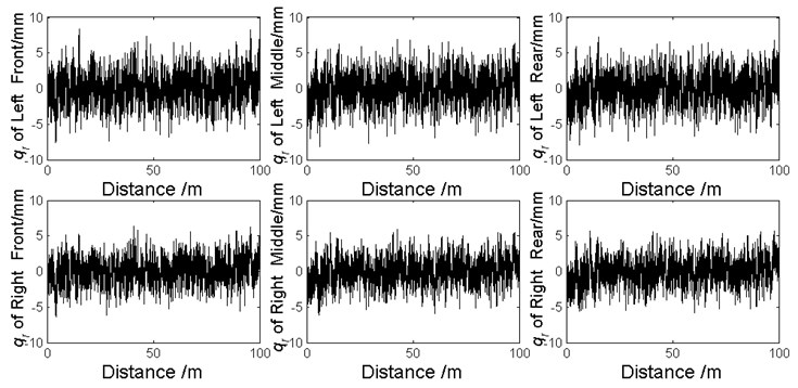
Based on the algorithm stated above, a six-wheel excitation model for dump truck is established via Matlab/Simulink. Take the class B road as an example. $G_q\left(n_0\right)=\text{64×1}{\text{0}}^{\text{-6}}{\text{m}}^{\text{3}}$, $B=$ 2 m, $L1=$ 3.8 m, $L2=$ 3.8+1.35 m, the vehicle’s velocity is $v=$2.78 m/s. The random road profiles for six wheels in space domain could be reached as shown in Fig. 1.

Fig. 1Random road profiles for six wheels of dump truck

2.2. The time-domain modelling of long-waved road profile

In order to quantitatively investigate the impacts of long-waved low-frequency road topography on the vehicle vibration and fatigue life of frame, it is necessary to superimpose deterministic long-waved bosses on the standard random road profile, taking standard road profile as both background and reference, to build a full-band asymmetric boss test road. Thus, by superimposing a set of bosses, the cross-section geometric parameters of which were known, an asymmetric undulating road sample similar to the real test road is built.

As it is shown in Fig. 2, long-waved road is constituted by several bosses placing on a class B road. The geometrical parameters of the boss cross-section are shown in Fig. 2(a). The lift (between O-A, which is 0-0.6 m) and return (between B-C, which is 1.2-1.8 m) trip of undulating road are all circular curves, whose radius are $R=$1.275 m, which respectively tangent to point A and B. The upper surface of the boss is a horizontal straight line, with $H=$0.15 m. The mathematical expression of the boss road profile can be given as follows:

8

$\left\{\begin{array}{ll}(x-0.6{)}^2+(q_B+(R-0.15){)}^2=R^2,& x=\left[0,\mathrm{}0.6\right],\\ q_B=0.15,& x=\left[\mathrm{0.6,1.2}\right],\\ (x-1.2{)}^2+(q_B+(R-0.15){)}^2=R^2,& x=\left[\mathrm{1.2,1.8}\right],\end{array}\right.$

where $x$ represents the distance along the test road, $q_B$ is the boss’s vertical ordinate at distance $x$. As shown in Fig. 2(b), bosses are arranged alternately left and right on the road. The longitudinal separation between every boss and the adjacency one to the other side is 0.85 m.

Fig. 2The research sample of long-waved road profile

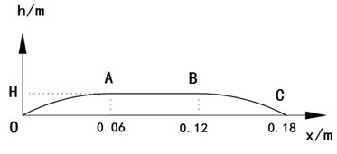
a) The geometrical parameters of the boss cross-section

b) The boss test road

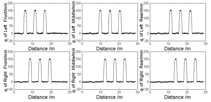
Combined with the random road profile $q_r$ gained in section 2.4, the full-band long-waved road profile $q_l$ to be reconstructed was given by the summation of Eqs. (2, 6-8). As shown in Fig. 3.

9

$q_l=q_r+q_B.$

Fig. 3The full-band long-waved road profile

3. The 11-DOF vehicle vibration model of dump truck

The entire system was modelled by the linear 11-degree of freedom (11-DOF) model comprising 3-DOFs associated with the vehicle body, 6-DOFs associated with the bounce and roll motions of three integral axles, and 2-DOF for the pitch motions of the balanced suspension.

This paper mainly studies the dynamic loads of frame bearing points. Therefore, the cab and other parts above the frame are simplified to the equivalent mass of the centroid point.

For most vehicles, resonances in roll occur at lower frequencies (typically between 0.5 and 1 Hz) than resonances in bounce (Gillespie [15]), which is easy to study the vibration characteristics of vehicle using the 1/2 model. However, the coherence of the left and right wheel tracks of asymmetric long-waved road tend to be smaller and the vehicle is more responsive to roll input. Therefore, it is necessary to establish the whole vehicle model rather than a pitch-plane model.

Three axles in 6×4 dump truck are all integral axles, where the axle is a kind of dependent suspension. There is a direct geometric relationship between bounce motions of left and right axle ends, which could not be simplified as two independent vertical degrees of freedom [8]. The dependent model must be introduced, as shown in Fig. 4.

Fig. 411-DOF vibration model of dump truck. Where, Zb is the bounce motion of vehicle body, θ is the pitch motion of vehicle body, and φ is the roll motion. Zi (i=1~6) represents the bounce motion of axle end. Zj (j=A, B, C, D) represents the bounce motion of frame bearing point. Zi and θi (i=f, m, r) are the bounce and roll motions of integral axle. Zj (j=E, F,G, H) represents the bounce of stabilizer rod end

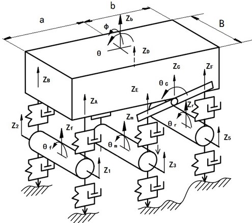
The balanced suspension has been widely utilized in three-axle dump truck to enhance the axle load; therefore, it is necessary to build a reasonable balanced suspension model and demonstrate its vibration characteristics [16]. As shown in Fig. 4, the leaf springs of the balanced suspension are regarded as a whole. The middle part of the leaf springs is connected with the sprung mass. Both ends of the leaf springs are separately linked with the front and rear axle through the rigid stabilizer rod. The front and rear axle's vibration are coupled together with the stabilizer rod.

The equation of motion of a linear vehicle model (with linear geometry and linear springs and dampers representing tire and suspension elements) can be written in matrix form as:

where $\mathbf{M}$ is the matrix representing vehicle body mass, $\mathbf{C}$ is a matrix of vehicle damping, $\mathbf{K}$ is the stiffness matrix of the vehicle system, ${\mathbf{C}}_{\mathbf{t}}$ is a matrix of tire damping, ${\mathbf{K}}_{\mathbf{t}}$ is the stiffness matrix of the tire, $\mathbf{Z}$ is the vector of vehicle dynamic responses and ${\mathbf{Q}}_{\mathbf{g}}$ is the vector of displacement inputs acting on the tires.

It was assumed that both the pitch angle and roll angle were so small that kinematical motions at the front axle, rear axle, second axle and balanced suspension mount might be approximated by the following equations, respectively:

Vertical bounce of axle ends could not be directly obtained because of the DOF definition of balanced suspension. Based on the small deflection hypothesis, the following equations could be approximately gained.

In order to simplify the solving for time-domain solution, to obtain a convenient and compact way to model and analyze systems with multiple inputs and outputs, the multivariable differential equations should be converted to the state space representation, which is a mathematical model of a physical system as a set of input, output and state variables related by first-order differential equations. To abstract from the number of inputs, outputs and states, the variables of linear and time invariant system are expressed as vectors, and the differential and algebraic equations can be written in matrix form. It is essential that the matrix and vector modeling is very efficient from a computational standpoint for computer implementation.

Consideration of the tire damping in vehicle vibration model will put time derivatives of road roughness in the right hand side of Eq. (10). Since most of the control theory is done for systems without considering the input derivatives, it is necessary to lower the order of inputs, i.e. to remove the time derivatives of inputs [17].

The conventional order reduction approach is a direct numerical differential operation to road roughness, to obtain time derivatives of road roughness. Firstly, the road roughness input ${\mathbf{K}}_{\mathbf{t}}{\mathbf{Q}}_{\mathbf{g}}+{\mathbf{C}}_{\mathbf{t}}{\dot{\mathbf{Q}}}_{\mathbf{g}}$ was directly converted to force input acting on the vehicle $\mathbf{f}\left(t\right)$ through numerical differential operation. Then Eq. (10) was recast into multivariable state space equations given by:

where $\mathbf{I}$ and $0$ represent identity and null matrices with similar dimensions as the property matrices, $\widehat{0}$ is a null column vector with a length similar to the forcing vector $\mathbf{f}$ and $\mathbf{x}$ is a vector containing the states (displacement and velocity vectors). And the state variables $\mathbf{x}$ was selected as Eq. (26):

Although input order reduction has been realized in Eq. (25) via the conversion from ${\mathbf{K}}_{\mathbf{t}}{\mathbf{Q}}_{\mathbf{g}}+{\mathbf{C}}_{\mathbf{t}}{\dot{\mathbf{Q}}}_{\mathbf{g}}$ to $\mathbf{f}\left(t\right)$, the essence of this order reduction is an approximate computational process of numerical differentiation algorithm based on Runge-Kutta. Order reduction itself could cause truncation error input and reduce the reliability and accuracy of system output. In order to oversimplify input vector, therefore, it is essential to keep input derivative for solving reliability and accuracy.

At present, the transformation from SISO differential equation containing input derivative to state space representation is achieved mainly by selecting an appropriate intermediate variable. Based on the SISO transformation method, the input, output variable and status variable are expanded to vector, variable of each system is expanded to coefficient matrix and matrix operations is introduced to the conversion process. Then, input derivatives of multivariable equations, ${\dot{\mathbf{Q}}}_{\mathbf{g}}$, could be eliminated successfully. State-space equation could be achieved, as shown in Eq. (27):

where the state variables $x_2$ was selected as Eq. (18):

Via a ss.m function in MATLAB, a 11-DOF state-space model of dump truck was constructed based on Eq. (27).

Based on the state-space model, then the responses of the dynamic system excited by the input $Q_g$ assigned by the time-domain road roughness in section 2.4 and 2.5 were simulated via the lsim.m function in MATLAB.

4. Numerical simulation and validation

The acceleration and load signals of specific/arbitrary position could be obtained via numerical simulation by the proposed state-space model. Before further calculations, the 11-DOF model needs to be validated and calibrated by comparing the simulated and measured vehicle responses.

4.1. Time-domain simulation of dynamic loads

The dynamic wheel load is defined as the tire load changes relative to static equilibrium. $F_{di}$ ($i=1,2,3,4,5,6$) is the dynamic tire load of each axle end in 11-DOF dump truck. Therefore, the six tire loads can be given by:

29

$\left\{\begin{array}{l}{F}_{d1}=K_{t1}\left(Z_1-q_1\right)+C_{t1}\left({\dot{Z}}_1-{\dot{q}}_1\right),\\ F_{d2}=K_{t2}\left(Z_2-q_2\right)+C_{t2}\left({\dot{Z}}_2-{\dot{q}}_2\right),\\ F_{d3}=K_{t3}\left(Z_3-q_3\right)+C_{t3}\left({\dot{Z}}_3-{\dot{q}}_3\right),\\ F_{d4}=K_{t4}\left(Z_4-q_4\right)+C_{t4}\left({\dot{Z}}_4-{\dot{q}}_4\right),\\ F_{d5}=K_{t5}\left(Z_5-q_5\right)+C_{t5}\left({\dot{Z}}_5-{\dot{q}}_5\right),\\ F_{d6}=K_{t6}\left(Z_6-q_6\right)+C_{t6}\left({\dot{Z}}_6-{\dot{q}}_6\right).\end{array}\right.$

Dynamic load of frame bearing point is the frame load changes imposed by bearing points. There are four bearing points for the 11-DOF dump truck frame: 2 points on front spring supports (F_SA and F_SB) and each point on left and right of suspension ($F_{SC}$ and $F_{SD}$). In Section 3.2, leaf spring of balanced suspension has been simplified to two springs, as shown in Fig. 4. The introduction of virtual stabilizer rod in the balanced suspension model results in the emergence of the intermediate variables, i.e., the hypothetical dynamic loads of stabilizer rod end, $F_{SE}$, $F_{SF}$, $F_{SG}$ and $F_{SH}$. The formula of front bearing points of frame and four dynamic loads of rod ends is shown in Eq. (30) and the relationship between dynamic loads of rod ends and that of balance shaft ends is shown in Eq. (31):

30

$\left\{\begin{array}{l}{F}_{SA}=K_1\left(Z_1-Z_A\right)+C_1\left({\dot{Z}}_1-{\dot{Z}}_A\right),\\ F_{SB}=K_2\left(Z_2-Z_B\right)+C_2\left({\dot{Z}}_2-{\dot{Z}}_B\right),\\ F_{SE}=K_3\left(Z_3-Z_E\right)+C_3\left({\dot{Z}}_3-{\dot{Z}}_E\right),\\ F_{SF}=K_5\left(Z_5-Z_F\right)+C_5\left({\dot{Z}}_5-{\dot{Z}}_F\right),\\ F_{SG}=K_4\left(Z_4-Z_G\right)+C_4\left({\dot{Z}}_4-{\dot{Z}}_G\right),\\ F_{SH}=K_6\left(Z_6-Z_H\right)+C_6\left({\dot{Z}}_6-{\dot{Z}}_H\right),\end{array}\right.$

31

$\left\{\begin{array}{l}{F}_{SC}=F_E+F_F,\\ F_{SD}=F_G+F_H.\end{array}\right.$

Generally speaking, the longitudinal force imposed by balanced suspension on vehicle frame is not significant when driving steadily on a class B road or above. When the road surface slightly undulates, which does not cause significant deflection of leaf spring, the longitudinal dynamic force generated by driving force fluctuations will be delivered to the 4th cross member and the bottom of balance shaft via traction bar.

The introduction of balanced suspension effectively improved load distribution between second and rear axles, moderated axle dynamic load shocks and enhanced axle service life. In the meantime, however, the structure principle of integral balanced suspension decides that, when the resultant force of longitudinal force components of front and rear axles does not equal to zero, the frame will suffer horizontal component force exerted by off-road road roughness. Computing conclusion shows that the root mean square of frame longitudinal dynamic load, under the excitation of the bosses road with $H=$0.15 m, can range up to 3 % to 5 % of that of vertical load, which cannot be ignored in analysis methods.

As it is shown in Fig. 5, long-waved road profile can cause the contact force between tire and ground deviating from vertical direction. The magnitude of horizontal component force depends on the angle between road profile and horizontal plane. The sum of vertical component forces of the second axle and rear axle equals to the burden of vehicle load on balance shaft, which is $F_C=F_{EV}+F_{FV}=F_{d3}+F_{d5}$. Whereas, the horizontal loads exerted by balance axle seat equal to the sum of component forces from two tires, which is $F_{Ch}=F_{Eh}+F_{Fh}$. During the transfer process from tire contacting force to frame bearing force, the leaf spring and traction bar all played a delivering role. The resultant force of frame exerted by balance shaft always follows the mechanical analysis conclusion stated above.

Fig. 5Mechanical analysis of balanced suspension

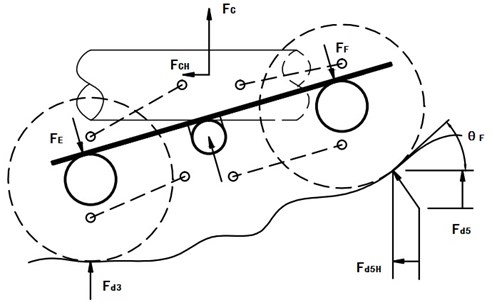
Equivalently shift the horizontal force delivered by traction bar to the axis of the balance shaft. The horizontal loads on two sides of balance shaft, $F_{CH}$ and $F_{DH}$, could be written as:

32

$\left\{\begin{array}{l}{F}_{CH}=F_{d3}\times \mathrm{t}\mathrm{a}\mathrm{n}{\theta }_E+F_{d5}\times \mathrm{t}\mathrm{a}\mathrm{n}{\theta }_F,\\ F_{DH}=F_{d4}\times \mathrm{t}\mathrm{a}\mathrm{n}{\theta }_G+F_{d6}\times \mathrm{t}\mathrm{a}\mathrm{n}{\theta }_H.\end{array}\right.$

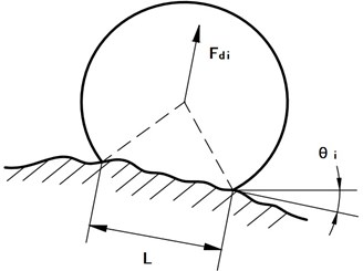
Considering the envelope effect from tire to road, the tire grounding angle could not be directly solved via simple derivation operation from road displacement. Contacting print of tire and road profile can be equivalent to a straight line, $L$. Then by calculating angle ${\theta }_i$$(i=E,F,G,H)$, as shown in Fig. 6, the more reliable tire grounding angle, ${\theta }_E$, ${\theta }_F$, ${\theta }_G$, ${\theta }_H$, could be obtained.

Fig. 6Tire grounding angle

4.2. Road tests for model validation

In order to make the comparison between the predicted and measured vehicle responses, under excitations of class B road and boss test road, two 30-meter-long test roads are chosen as the road samples. As shown in Fig. 3(b).

The parameters of the test vehicle are shown in Table 1.

Table 1Parameters of the 6×4 dump truck

Curb weight / (kg)	12815	Front spring stiffness / (N/m)	3.8×105	Front tire stiffness / (N/m)	1.1×106
Wheelbase / (mm)	3800+1350	Rear spring stiffness / (N/m)	3.6×106	Rear tire stiffness / (N/m)	2.2×106
Track / (mm)	1850	Front axle damping / (N s/m)	10000	Front tire damping / (N s/m)	3500
		Suspension damping / (N s/m)	2000	Rear tire damping / (N s/m)	7000

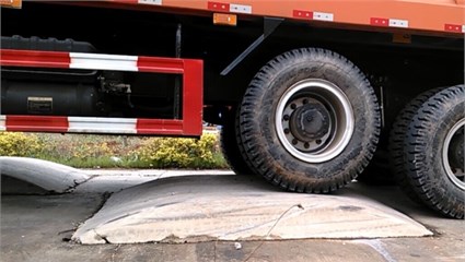
As shown in Fig. 7, in order to acquire the dynamic loads of the front wheels, two wheel force transducers were installed on each side of front axle (Suzhou Brontek Measure & Control Technology Co., Ltd, Model No. SD823). For acquiring the acceleration signals of axle ends and frame bearing points, to verify the second-order response output of the 11-DOF model, acceleration sensors were installed near the leaf springs of front and rear axles, and on the main frame near the installing seat of balance shaft (Sinocera Piezotronics, Inc., Model No. X901).

Fig. 7Sensor arrangement

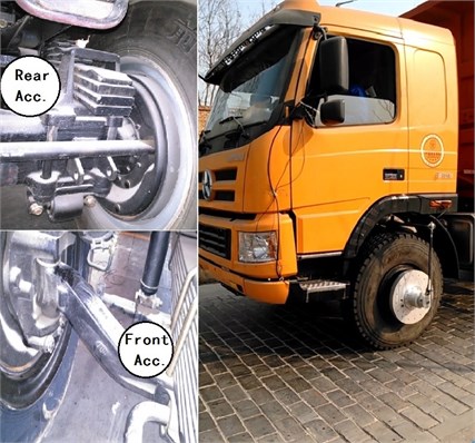
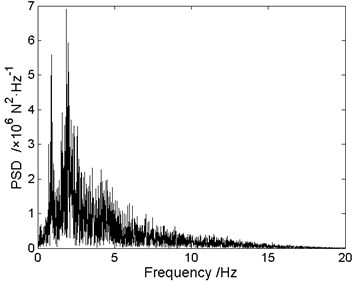
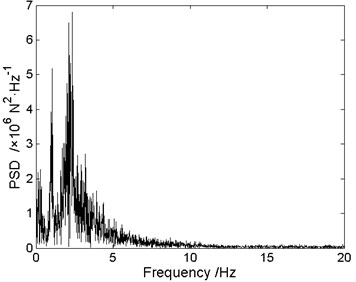
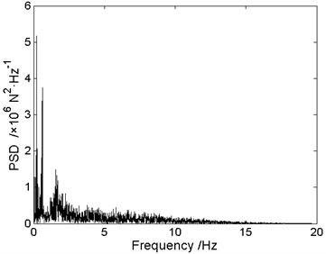
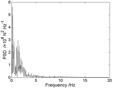
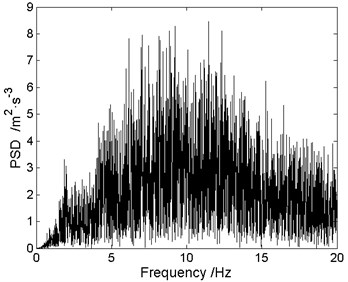
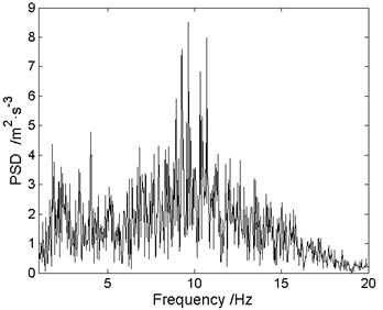
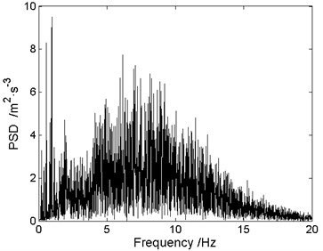
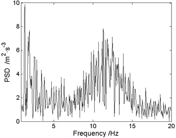
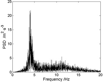
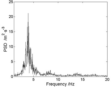
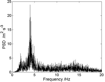
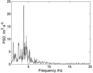
Fig. 8Power spectral density (PSD) of front wheel load (Fd1), acceleration of front axle (AccF) and acceleration of balance shaft seat (AccBS) under two road profiles

a) PSD of simulated Fd1 under class B road

b) PSD of measured Fd1 under class B road

c) PSD of simulated Fd1 under long-waved road

d) PSD of measured Fd1 under long-waved road

e) PSD of simulated AccF under class B road

f) PSD of measured AccF under class B road

g) PSD of simulated AccF under long-waved road

h) PSD of measured AccF under long-waved road

i) PSD of simulated AccBS under class B road

j) PSD of measured AccBS under class B road

k) PSD of simulated AccBS under long-waved road

l) PSD of measured AccBS under long-waved road

Fig. 8 shows that, from the perspective of energy distribution in the frequency domain, the simulated results are well consistent with the measured data, which proves that the proposed time-domain vehicle model can well describe the dynamic characteristics of dump truck.

Fig. 8(a-b) and 8(c-d) show that the PSD peak of Fd1 (front wheel load) near the 2.5 Hz, corresponding to sprung mass motion, has been distinctly restrained. Whereas, the low frequency component corresponding to front-axle unsprung mass is released, and shows an obvious aggregation in low frequency band. It presents that under long-waved road excitation, front suspension is more susceptible to low frequency road, and the influence from sprung mass motion has been correspondingly weakened. The PSDs of acceleration signals show the similar conclusions, as shown in Fig. 8(e-f) and 8(g-h).

As shown in Fig. 8(i-j) and 8(k-l), the PSDs of acceleration on balance shaft seat under different road profiles show a higher consistency, which proves that the balanced suspension can well absorb the shock to frame caused by long-waved road profile, and eases the low-frequency vibration of balance shaft seat.

The delicate difference lies in the aggregation of responding load between 2-5 Hz caused by asymmetrical long-waved road, which illustrates that roll motion caused by asymmetrical road could not be restrained by the balanced suspension. In other words, the influence of roll motion to balanced suspension vibration mainly embody at 2~5 Hz.

5. Fatigue life analysis

According to Eq. (20-22), six load-time histories of frame bearing points, loads of balanced suspension seat containing vertical load and horizontal load, could be gained. After a series of pre-processing, the load-time histories were imported into the fatigue life calculation and damage analysis software, nCode, to anticipate and analyze fatigue life of frame. Several conclusions are drawn as follows.

Fig. 9The relationship among the fatigue life of weak area, wave amplitude and wavelength ratio in total distance

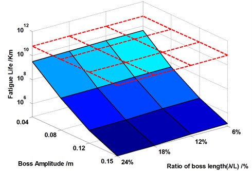
In order to make a quantitative research on influence of parameters of long-waved road to fatigue life of frame, take the wave amplitude, $H$ and the ratio of wavelength to total distance, $\lambda /L$, as variables separately and take responding loads under various road profile as the inputs for fatigue life calculation. The relationship among the fatigue life of weak area, wave amplitude and wavelength ratio can be drawn as Fig. 9.

Wherein, the red dashed line, between 10¹⁰ and 10¹² km, is the frame fatigue life under class B road, which is treated as the life criterion for research on other working conditions.

As shown in Fig. 9, fatigue life of frame is shortened linearly with proportion of boss length in total distance increasing. Nevertheless, with the increase of boss amplitude, the shortening of fatigue life shows a logarithmic trend. Therefore, in Fig. 9, the logarithmic scale is adopted in vertical coordinate.

Take the road with amplitude = 0.12 m as an example, when the ratio of boss wavelength increases from 6 % to 24 %, fatigue life of fatigue weak area decreases from 1.391×106 km to 9.212×105 km. And the linear correlation coefficient of four ratios is 0. 9841. Under excitation of different boss amplitudes, $H=$0.15 m, 0.08 m and 0.04, the other three working conditions show the similar linear correlation conclusion, whose linear correlation coefficients are 0.9859, 0.9776 and 0.9639 respectively.

The logarithmic relationship, shown by fatigue life of weak area under different amplitudes, demonstrates that the impact of amplitude of long-waved road is more obvious than that of ratio on fatigue life of frame.

Fig. 10The fatigue life contour of frame under class B road excitation

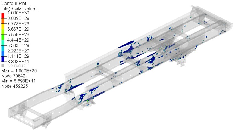
Fig. 11The fatigue life contour of frame under long-waved road sample 1 (H= 0.04 m)

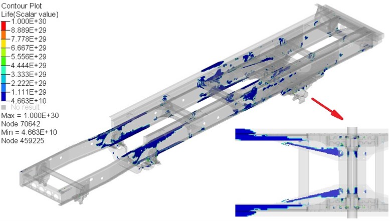
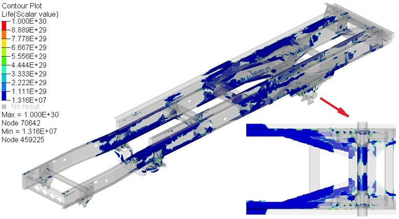
Fig. 12The fatigue life contour of frame under long-waved road sample 2 (H= 0.12 m)

It can be seen from Fig. 9 and Fig. 10, compared to the fatigue life contour under class B road, the fatigue weak area of frame under long-waved road ($H=$0.04 m, ratio of wavelength is 24 %) has become decentralized mainly to two parts. The one is on main frame side rail near the engine supporting beam and the other is between the third crossmember and front end of main-sub frame connecting plate. These fatigue analysis results are consistent with the statistical conclusions of frame fatigue cracking under mining and construction site [18].

In order to investigate the impact of wave amplitude on frame fatigue life, on the premise of same wavelength ratio, another long-waved road sample and its corresponding load-time histories were created. Then the fatigue life of frame under the excitation of higher amplitude roads was calculated and analyzed.

As shown in Fig. 13, under the excitation of the second long-waved road sample, whose boss amplitude is 0.12 m, the fatigue life of frame is shortened dramatically and the fatigue weak area began to expand to rear of frame. It can be seen from the bottom view of balanced suspension in Fig. 10 and Fig. 11, with the increase of the wave amplitude, the fatigue weak area of fourth crossmember and balance shaft assemblies increased significantly. The fatigue weak area of other regions did not show much obvious positional deviation, which indicates that the impact of wave amplitude change on frame fatigue life is mainly focused on the main frame near the third crossmember and balance shaft assemblies.

6. Conclusions

This work was aimed at investigating the impacts of long-waved road roughness on fatigue life of dump truck frame by establishing 11-DOF vibration model considering tire damping, dependent suspension and balanced suspension.

1. Introduction of matrix operations makes the transformation method of single input single output (SISO) differential equation containing input derivative to state space representation successfully expand to the multivariate equations (MIMO). Therefore, 11-DOF dump truck model has been successfully established considering tire damping, on the premise of not introducing truncation error. The model has been validated and calibrated via dynamic wheel forces and acceleration signals of axle end collected in road tests. From the perspective of energy distribution of the signal in the frequency domain, the simulated results are basically consistent with measured data, which proves that the proposed time-domain vehicle model could well describe the dynamic characteristics of dump truck.

2. Under the long-waved road excitation, front suspension is more susceptible to low frequency road roughness, rather than the sprung mass motion. The balanced suspension can well absorb the shock to frame caused by long-waved road profile and ease the low-frequency vibration of balance shaft seat. Whereas, the balanced suspension structure cannot well suppress the roll motion caused by asymmetrical road.

3. The calculation results show that fatigue life of frame is linearly shortened with the ratio of boss length in total distance increasing. Nevertheless, with the increase of boss amplitude, the shortening of fatigue life shows a logarithmic trend, which demonstrates that the impact of amplitude of long-waved road is more obvious than that of ratio on frame fatigue life.

4. Simulated analysis of frame fatigue life demonstrates that under long-waved road excitation, the fatigue weak area is more decentralized to two parts. The one is on main frame side rail near the engine supporting beam and the other is between the third crossmember and front end of main-sub frame connecting plate. The further analysis shows that the increase of long-waved road amplitude will lead to the fatigue weak area expanding to the back part of frame. The change of long-waved road amplitude has an influence on fatigue life, mainly focused near the third crossmember on the main frame and balance shaft assemblies.

The simulation conclusions and the statistical results of frame fatigue cracking in actual mining area and construction site have a higher consistency, which fully supports the reasonability of this paper.