Abstract
An approach of structural response reconstruction for non-proportionally damped systems is proposed in this paper, which is a time domain method based on the empirical mode decomposition method with intermittency criteria and modal superposition method. The state space method is employed for decoupling the dynamic system equation to obtain the complex mode shapes. Response reconstruction of the structural system in the presence of closely spaced modes is studied in detail. The key idea is to regard each set of closely spaced modes as an integral part. Two numerical examples are conducted to validate the effectiveness of the proposed method.
1. Introduction
Structural dynamic response reconstruction has received increased attention in the past decades. In order to monitor the structure's condition, it is necessary to accurately obtain the system response in the critical areas of the structure [1, 2]. However, in some instances, it is not possible to measure the responses at the desired locations in operational conditions [3]. For example, the locations of interest are at interface between substructures in a large structural system [4]. In addition, in real life, it is impossible to arrange sensors at every location due to economic reasons. Therefore, prediction of the dynamic responses at critical spots becomes an essential component to perform structural monitoring [5, 6].
Literature review on recent studies reveals several types of approaches for structural dynamic response reconstruction. One type is based on transmissibility concept [7, 8]. Ribeiro et al. [9] defined the concept as a transmissibility matrix between the known response functions and the other unknown response functions in frequency domain. The transmissibility matrix allows for the reconstruction of the response at an arbitrary location of the structure from another location where the response is known. Its basic idea is transforming the measurable responses into the responses at the desired locations with a transmissibility matrix. Law et al. [10] proposed the concept of transmissibility for dynamic response reconstruction in a substructure, and expanded the concept of transmissibility to the wavelet domain using the unit impulse response function [11, 12]. However, for all the applications using transmissibility concept, it is necessary to know the locations where forces or moments are applied.
The second type of the reconstruction methods is based on the empirical mode decomposition (EMD) [13]. For convenience, this method is called the REMD (reconstruction based on EMD) method for short in this paper. Responses of the measurable locations are decomposed into modal responses represented in intrinsic mode functions (IMFs). Using those modal responses, the modal responses at inaccessible locations are computed with the mode shapes. Then modal superposition methodology is employed to calculate the dynamic responses in time domain with all the modal responses. To ensure each IMF contains only one frequency component, the sifting process with intermittency criteria is used. This method is very efficient in terms of computational cost, and very suitable for various dynamic response reconstruction based on the different types of sensor measurements. Also a limited number of measurement locations are required. Another advantage of this response reconstruction method is that there is no longer a need to know the locations where the excitation forces are applied, compared with the reconstruction method based on transmissibility concept. However, due to the hypothesis of the intermittency criteria, when one mode couldn’t be separated accurately, especially when facing closely spaced modes [13], the REMD method will be no longer suitable. It has been marked as a challenge for a structure identification and reconstruction problem involving closely spaced modes [14]. In Ref. [15], the authors proposed a reconstruction approach based on the REMD method to deal with the situation of closely spaced modes. Using this method, there is no need to obtain the modal responses of the individual closely spaced modes. A complete mode set of a structure is divided into two sets: One set is the closely spaced modes, and the other set is the rest of the modes. The rest of the modal responses whose response are measurable can be obtained using the EMD method with intermittency criteria, and the rest of the modal responses at desired locations can be computed from them with the mode shapes. Thus, the contribution of the closely spaced modal responses can be obtained by the mode shapes and the rest of the modal responses.
Aside from the above methods, some other types of the methods have also been developed. In Ref. [16], the reconstruction problem is defined as an inverse optimization problem subject to constraints. Then sophisticated optimization techniques are adopted. In Refs. [17, 18], the dynamic reconstruction method of a flexible beam has been studied. It is based on the interpolation of available measurements using spline shape functions. The accuracy of reconstructed responses increases with the number of recorded sensors and is strongly influenced by the layout of sensors. Compared with these methods, the REMD method doesn’t need sophisticated optimization techniques and a lot of measured locations.
In a previous report by the authors [15], only the proportionally damped system was considered. Modes of proportionally damped systems preserve the simplicity of the real normal modes as in the undamped case [19]. However, there is no physical reason why a structural system should behave like this. In fact, practical experience in modal testing shows that most real-life structures possess complex modes, which indicates that the general linear systems are non-proportionally damped. In this paper, a reconstruction approach for non-proportionally damped system is developed, which is the extension version of Ref. [15]. The state-space method [20, 21] is the most popular method for decoupling the dynamic system equation, and it is employed in this paper for obtaining the complex mode shapes. The case of closely spaced modes is considered in detail. Furthermore, the case of multiple sets of closely spaced modes is also investigated.
2. Modal response using empirical mode decomposition
An essential step of the proposed dynamic response reconstruction method is to obtain the individual modal responses of the measured signals. The EMD method with intermittency criteria is adopted to decompose the measured signals into modal responses which are called IMFs in EMD. In Section 2.1, the standard sifting process of the EMD method [13, 22] is discussed. Section 2.2 describes the intermittency criteria.
The idea of the EMD method is to break down a given signal into functions which form a complete and nearly orthogonal basis for the original signal. The resulting functions, which have a mean value of zero and only one extreme between zero crossings, known as IMFs, are sufficient to describe the underlying dynamics of the signal. The sufficiency and completeness of the EMD method are ensured by the way the signal is decomposed [23]. Those approximately orthogonal constituent IMFs bear close resemblance to base functions and are problem specific and data oriented [24].
2.1. Sifting process of the EMD method
A sifting process is used by the EMD method to filter out IMFs from a given signal. is denoted as a time domain signal, the sifting process is summarized as follows: [13, 14, 22].
1. Construct the upper and lower envelopes of the signal by cubic-spline fitting. Compute the mean of both envelopes, which is denoted by .
2. Compute the first component and check to see whether is a monocomponent, referred to as an IMF. If it is not an IMF, continue the sifting process using as the new signal data.
3. Construct the envelops of and denote as the mean of the envelops, and compute the component .
4. Repeat step 3 for times until the resulting () is an IMF.
5. Denote , which is the first IMF extracted from the signal data.
6. Repeat the above steps to get the second IMF from the remaining signal of .
7. Continue the above procedure to obtain another IMF from the remaining signal until the rest of the signal () is the mean trend (or a constant) of the signal. is the th IMF and is the residue.
2.2. The EMD method with intermittency criteria
IMFs obtained from the sifting process described above may contain more than one frequency, which is not an exact modal response. To obtain the structural modal responses, the intermittency criteria are used to ensure that each of the IMFs contains only one frequency component. The idea of the intermittency criteria in sifting process is to remove all frequency components lower and higher than (an intermittency frequency) from an IMF by using a band-pass filter [13, 14, 25]. Here, is just determined by the th natural frequency of the structure. The procedure to obtain the modal responses is summarized as follows:
1. Estimate an approximate frequency range for (i.e. ) either by Fourier spectra of the measured signal or FEM computations as the band-pass filter.
2. Process the signal through the band-pass filter.
3. Use the sifting process described in Section 2.1 to process the data obtained from step 2. The first IMF is considered to be the approximation of modal response.
By repeating the above procedure with different frequency ranges for different natural frequencies, all the required modal responses can be obtained. It is important to note that the phase shift of the band-pass filter should be as small as possible. Using the sifting process with intermittency criteria, the original signal expression can be written as:
where is the modal response (that is also an IMF) for the th mode. (1,…, ) are other IMFs but not modal responses.
Applying the EMD method with intermittency criteria to the measured signal, the modal responses can be extracted except for the closely spaced modal responses which the band-pass filter cannot separate.
3. Reconstruction theory
In Ref. [13, 15], the modal superposition method was employed in response reconstruction, and only proportionally damped system was discussed. However, in real life, the general linear systems are non-proportionally damped. When the system is non-proportionally damped, the general equation of motion can’t be decoupled to second-order uncoupled equation by using real mode shapes in the undamped case. The state-space method is one of the most popular methods to solve the decoupling problem for the non-proportionally damped system according to the literature and it is based on transforming the second-order coupled equation into a set of 2 first-order coupled equations by augmenting the displacement response vectors with the velocities of the corresponding coordinates.
The general equation of motion of a viscously damped structure with DOFs can be written as:
where , and are the mass, damping and stiffness matrices of the structure, respectively; , , are, respectively, the nodal acceleration, velocity and displacement vectors of the structure; is the load vector. In state space, Eq. (2) can be expressed as:
Eq. (3) can also be simplified as:
where is the state vector, , are the matrices which are consisted of the system parameters, and is the vector of the excitation force. Obviously, Eqs. (3) and (4) are 2×2 first-order equations. According to the theory of the state-space method, the mode shape matrix can be obtained by solving the generalized eigenvalue problem as:
where is the complex mode shape, and the superscript “” represents the conjugation and is the complex eigenvalue. The mode shape matrix is expressed as:
3.1. Response reconstruction without closely spaced modes
Assume that the response of the structure doesn’t contain any closely spaced modes. According to the theory of modal analysis, the response can be expressed as the summation of modal responses. Define that , (regard as the responses of DOF- and DOF-) are the two responses of the known responses which can be obtained by sensor measurement, is the vector of the unknown responses one wishes to know. The following equations can be obtained as:
where the subscript represents the th mode, and represents the mode information for the th DOF under th mode. represents the mode information for the DOFs whose responses are unknown. is the response of the mode in modal coordinate, and is the th modal response for DOF- in generalized coordinate. From Eqs. (7) and (8), we have:
Substituting Eq. (10) into Eq. (9), the following equation can be obtained as:
with the matrix and the vector , which are respectively defined as:
where can be computed by using the EMD method discussed in Section 2, and can be obtained using the FEM. According to Eq. (11), it can be concluded that the unknown responses, e.g. at sensor inaccessible locations, can be computed from one response at a measurable location. Additionally, the exact mode shape is obtained from an accurate FE model for all the cases studied. Under realistic conditions, the estimated mode information from measurements or an inaccurate finite element model may be induced uncertainties in the reconstruction results [15].
3.2. Response reconstruction in the presence of closely spaced modes
When a structure exists with closely spaced modes, the method proposed in Section 3.1 will be not suitable for the response reconstruction of this structure. In this section, an improvement to the reconstruction method is proposed to handle this situation with closely spaced modes.
Assuming that th and th modes are closely spaced, the subscripts and represent the information of the closely spaced modes and the rest of the modes, respectively, the subscript and represent the information of the DOFs whose responses are known and unknown, respectively. The known-set and unknown-set responses can be written as:
where is the closely spaced mode shape matrix of the DOFs- at which responses are known, is the rest of the mode shape matrix of the DOFs-. and are the closely spaced mode shape matrices of the DOFs- and DOFs-. and are the response vectors of the closely spaced modes and the rest of the modes in modal coordinate, respectively. They can be written as:
in which and are the responses of the two closely spaced modes in modal coordinate just as assumed before. , ,…, are the responses of the rest of the modes in modal coordinate, respectively.
From Eq. (14), the responses of the closely spaced modes in modal coordinate can be obtained as:
where denotes the pseudo-inverse of matrix . It is should be noted that the number of the known responses should be at least 2 times equal or greater than the number of the closely spaced modes.
Substituting Eq. (18) into Eq. (15), the vector of unknown responses can be written as:
For Eq. (19), there are two methods to obtain the unknown responses vector . One is to compute directly using the EMD method, but it is more complicated than the following method, because it requires executing the EMD method for all of the known responses according to Eq. (19). The algorithm is illustrated in the following text.
Eq. (19) can be transformed into another form as following:
and several matrices are defined as:
in which the subscript represents the information of DOF- at which response is known, the subscript ,…, represent the information of the rest of the modes, and is denoted as the vector of the rest of the modal responses of DOF-. Therefore, Eq. (20) can be expressed as:
, and can be derived by FEM, and can be computed by the EMD method with intermittency criteria. Eq. (25) can be called the reconstructed equation, and it is the same formulation as Eq. (21) in Ref. [15]. Note that a restriction of this proposed method is the number of the known responses must be greater or equal than the number of closely spaced modes .
When a structure contains multiple sets of closely spaced modes, Eq. (14) can be written as:
where represents the set of closely spaced modes, and is the corresponding modal responses of the known responses, which just can be obtained by the EMD method according to Fourier spectra. Then one can obtain that:
Eq. (15) can be easily transformed as following:
where:
Eq. (28) is also the reconstruction equation for the case of multiple sets of closely spaced modes. Note that the number of DOFs must be greater or equal than the number of 2× modes due to the pseudo-inverse of matrix . Taking each set of closely spaced modes as an integral part to obtain the modal responses is the key idea for dealing with this situation.
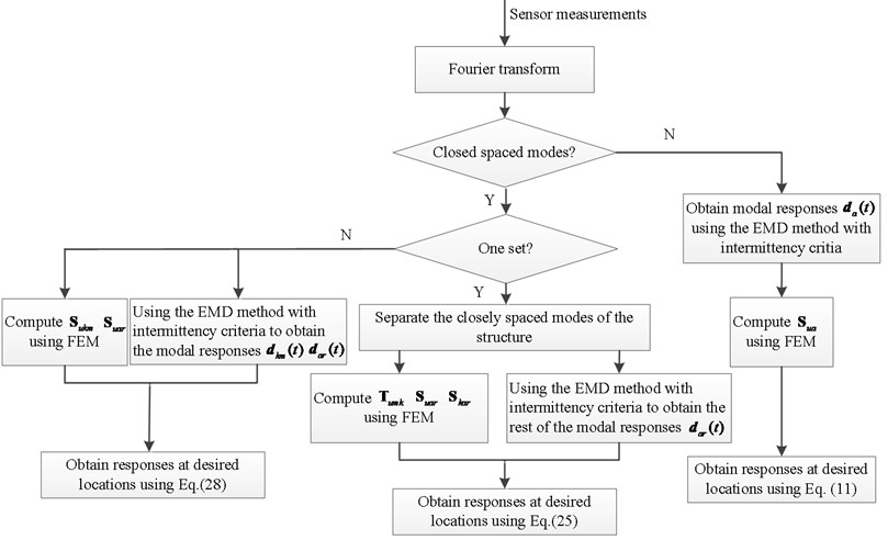
For stochastic or transient excitation, such as vibrations induced by ambient wind and earthquakes, the proposed method can reconstruct dynamic responses accurately and rapidly. Fig. 1 presents the overall reconstruction procedure for the methods presented in Section 3.1 and 3.2.
It should be noted that the method based on the modal superposition method presented in Section 3.1 and 3.2 are suitable for stochastic and transient excitation, and also for the process of both free vibration and steady forced vibration. Moreover, this proposed method is suitable for various types of dynamic responses, not only displacement responses but also velocity and acceleration responses.
Fig. 1Overall procedure of response reconstruction for non-proportionally damped system
4. Numerical examples
Two numerical examples are presented here. The first example is about a 3-DOF model, which is to verify the method of response reconstruction for the structure without closely spaced modes. The second example is based on a structural system of a 6-DOF mass-spring, which is to verify the reconstruction method in the presence of closely spaced modes.
4.1. Example 1: Response reconstruction without closely spaced modes
A 3-DOF theoretical model is used in this example. The mass, stiffness and damping matrices are presented as following:
The units are tone, N/mm and N/mm/s, respectively. No excitation force is applied, i.e. free vibration. The method proposed in section 3.1 is used to reconstruct the unknown responses. The displacement responses of DOF-1 and DOF-2 are used to be decomposed into modal responses (as ) by the EMD method.
The sampling frequency is 100 Hz, and the sampling time is 20 s. Fig. 2 shows the known displacement response of DOF-1. The Fourier spectra of the response is plotted in Fig. 3 where the three order frequencies are shown. The performance of the REMD method depends on the ability of the band-pass filter to separate different modes. Table 1 gives frequency ranges for each band-pass. Fig. 4 presents the filtered results of the rest of the modal responses. The reconstruction result and the theoretical prediction of DOF-1 are illustrated in Fig. 5. Fig. 6 is the partial time-history chart of Fig. 5 from 2 s to 10 s. From the two figures, it can be observed that the reconstruction result obtained from the proposed method is very close to theoretical prediction except for the beginning region. The discrepancy at the beginning of Fig. 5 is possible a result of the end boundary effect, which has been wildly discussed in literature as the intrinsic weakness of EMD [20]. This example proves that the proposed method is suitable for response reconstruction for free vibration.
Fig. 2Displacement response of DOF-1 with no noise terms
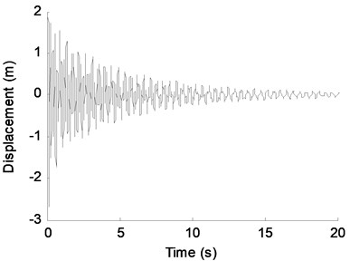
Fig. 3Fourier spectra of displacement response of DOF-1
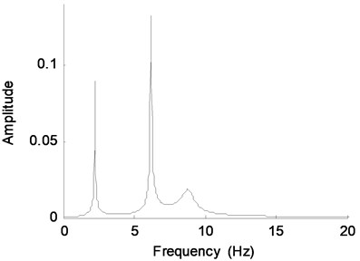
Fig. 4The modal responses of DOF-1 obtained using the EMD method with intermittency criteria
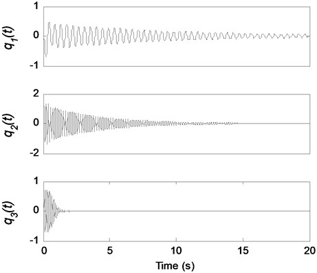
Fig. 5Theoretical response and reconstructed response (using the REMD method) of DOF-3
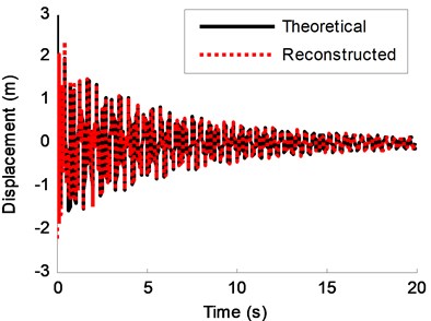
Fig. 6Zoom-in view of a segment (2-10 s) of Fig. 5
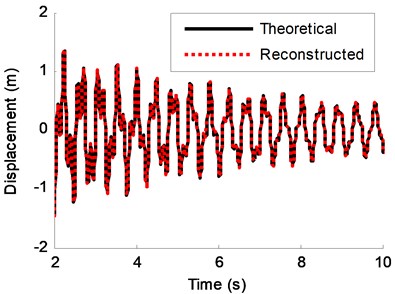
Table 1Frequency ranges for each band-pass filter
Mode | I | II | III |
Natural frequency | 2.24 | 6.28 | 9.06 |
Passband corner frequency (Hz) | [0.5-1.6] | [4-5] | [8-8.5] |
Stopband corner frequency (Hz) | [3-4] | [7.2-8] | [9.3-9.8] |
4.2. Example 2: Response reconstruction in the presence of closely spaced modes
A six DOF mass-spring system, as shown in Fig. 7, is presented here to demonstrate the overall reconstruction procedure for the problems which involving closely spaced modes. And its characteristics are described in Table 2. Liang damping [26] is used in all the simulations of example 2, which is defined as:
where . It is easily verified that non-proportional damping ensures with the simple equation:
Table 3 shows the damping coefficients and the information of external excitations for all the cases.
Fig. 7The 6DOF model used in the simulations. Liang damping C=αM+βK+R is used
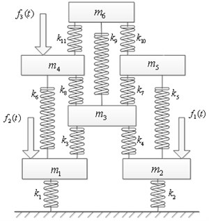
Table 2Characteristics of the structure system
7 | 7 | 4 | 13 | 12 | 8 | |||||
1 | 1 | 2 | 8 | 9 | 10 | 2 | 4 | 12 | 16 | 16 |
Unit: mass-kg stiffness-105 N/m. Liang damping is used for all the cases | ||||||||||
Table 3Information for different cases
Example | Case | Description | Damping coefficient | Excitation |
Example1 | – | No closely spaced modes | Direct damping matrix | Free vibration |
Example2 | Case 1 | Closely spaced modes | 1, 1e-5 | |
Case 2 | Effect of noise level | 1, 1e-5 | ||
Case 3 | Effect of high damping ratio | 1, 1e-4 | ||
Case 4 | Effect of multiply stochastic forces | 1, 1e-5 | , | |
Case 5 | Two sets of closely spaced modes | 1, 1e-5 | ||
: transient force. , : stochastic force | ||||
4.2.1. Case 1: Basic example
Sinusoidal excitation force is applied at DOF-2 for a duration of 0.05 s, which is:
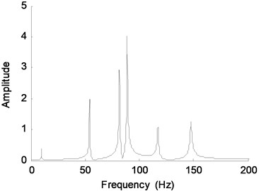
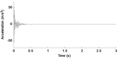
The sampling frequency is 2000 Hz. Fig. 8 shows the known acceleration response of DOF-4 with no noise terms. The Fourier spectra of the response is plotted in Fig. 9 where the six theoretical natural frequencies are shown. It is observed that the 3rd and 4th modes are closely spaced. So the number of the known responses should be at least equal to 4 to satisfy the relationship of .
Fig. 8Acceleration response of DOF-4 with no noise terms
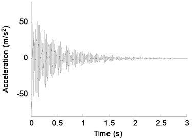
Fig. 9Fourier spectra of acceleration response of DOF-4
The method proposed in Section 3.2 is used to reconstruct the unknown responses. It is assumed that the responses of DOF-1, 3, 4 and 6 are known. So the vectors of known and unknown responses are represented as:
The vectors of the responses in modal coordinate of the system can be written as:
The response of DOF-3 and 4 are used to be decomposed into modal responses to transfer the rest of the modal responses for the overall reconstruction procedure, i.e. , , according to Eqs. (21)-(24), the four critical matrices can be obtained as:
Thus, the unknown responses are easily computed associated to Eq. (25).
The modal responses of the rest of the modes which actually consisted of 1st, 2nd, 5th and 6th modes at DOF-3 and 4 are obtained by the EMD method with intermittency criteria. These four modal frequencies are used to design the band-pass filters. Frequency ranges for each band-pass filter are shown in Table 4. It is noted that the band-pass filter should have as small phase shift as possible [16]. Fig. 10 presents the filtered results of the rest of modal responses at DOF-4.
Table 4Frequency ranges for each band-pass filter
Mode | I | II | V | VI |
Natural frequency | 9.77 | 54.12 | 118.46 | 150.31 |
Passband corner frequency (Hz) | [6-9] | [45-52] | [102-114] | [132-140] |
Stopband corner frequency (Hz) | [10.5-13] | [56-62] | [119-130] | [160-170] |
Fig. 10The rest of the modal responses of DOF-4 obtained using the EMD method with intermittency criteria
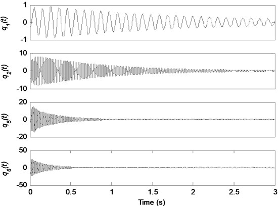
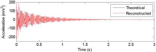
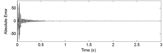
Fig. 11a) Theoretical response and reconstructed response of DOF-5, b) Absolute error between the theoretical response and reconstructed response of DOF-5
a)
b)
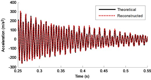
All of the unknown responses can be obtained based on the reconstructed equation, i.e. Eq. (25). For example, the reconstructed acceleration response and the theoretical response of DOF-5 are shown in Fig. 11(a), and Fig. 11(b) shows the absolute error of these two signals. Fig. 12 is the partial time-history chart of Fig. 11(a) from 1 s to 1.3 s. The two curves of responses are almost overlapping, indicating very high reconstruction accuracy of the proposed method. Also from Fig. 11 and Fig. 12, it is observed that the reconstruction result is very close to theoretical prediction except for the beginning region. At the beginning of Fig. 11(b), the periodic sinusoidal force introduces a frequency component (45 Hz) in the Fourier spectra, which is not the natural modes of the structure itself, and the contribution of 45 Hz is significant in frequency domain with the force applied. On the other hand, the discrepancy at the beginning of Fig. 11(b) is possible a result of the end boundary effect, which just like the discrepancies found in example 1. This case proves that the proposed method is suitable for response reconstruction with transient excitation. Following this basic example, effects of the noise level, high damping ratio, multiple stochastic forces and two sets of closely spaced modes are studied as four cases in detail.
Fig. 12Zoom-in view of a segment (1-1.3 s) of Fig. 11(a)
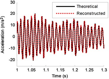
Fig. 13Theoretical response and reconstructed response of DOF-2 (no noise)
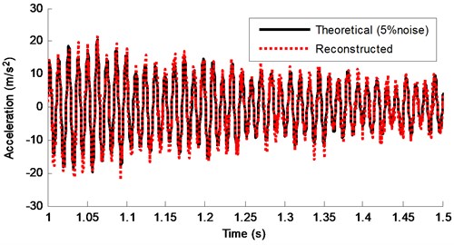
4.2.2. Case 2: Effect of noise level
To investigate the effect of the noise level on the performance of the reconstruction method, numerical experiments with different noise levels are performed. The noise is defined as a normally distributed random noise with zero mean and unit standard deviation, which can be written as:
where is the added noise to the original measured signal; is the noise level; is a standard normal distribution vector with zero mean and unit standard deviation and is the standard deviation of the original measured response.
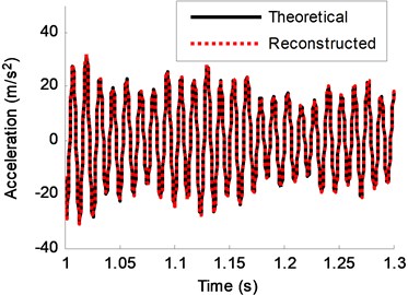
In this case, the acceleration response of DOF-2 is reconstructed using the known acceleration responses. Three noise levels are calculated (0, 2 %, 5 %). The reconstruction results are shown in Fig. 13-15. It can be seen that the noise level increasing leads to a bigger discrepancies. However, all of the reconstruction curves are still very close to the theoretical predictions. Two kinds of error are used to measure the error between the theoretical value and the reconstruction value. The mean absolute error (MAE) and relative error (RE) of a reconstructed signal are defined as:
Respectively, where is the length of the reconstructed series, and is the reconstructed value at time index and is the theoretical value of the signal. MAE and RE values of the reconstructed responses under different noise levels are listed in Table 5. These two types of errors are very small that proving the high stability of the proposed method in the presence of measurement noise.
Fig. 14Theoretical response and reconstructed response of DOF-2 (2 % noise)
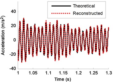
Fig. 15Theoretical response and reconstructed response of DOF-2 (5 % noise)
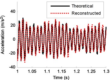
Table 5MAE and RE (%) values of each DOF in the response reconstruction under different noise levels
Noise level (%) | Error | DOF number | |
2 | 5 | ||
0 | MAE | 1.61 | 0.76 |
RE | 2.75 | 2.53 | |
2 | MAE | 2.11 | 1.28 |
RE | 6.26 | 2.64 | |
5 | MAE | 3.17 | 2.21 |
RE | 7.48 | 3.42 | |
4.2.3. Case 3: Effect of high damping ratio
Fig. 16Acceleration response of DOF-4 with high damping ratio
To investigate the effect of high damping ratio to the performance of the proposed response reconstruction method, a higher damping coefficient is used in this numerical case. The stiffness damping coefficient is taken as 1.0e-4 (10 times than before). Fig. 16 shows the acceleration response of DOF-4. The amplitude of the signal reduces rapidly due to the high damping ratio. Fig. 17 shows the theoretical prediction and reconstructed result of DOF-2. Fig. 18 is the zoom-in view of a segment (0.2 s-0.5 s) of Fig. 17. MAE and RE values of the reconstructed responses under different damping levels are listed in Table 6. It can be seen that RE of high damping system are larger than low damping system, however, all errors are very small, and the maximum RE is only 5.13 %. MAE of high damping system are less than low damping system due to the less absolute value of high damping system. From these figures and Table 6, good agreement can be observed between the theoretical acceleration and the reconstructed acceleration. This indicates that the proposed method has the capability for handling high damping ratio case.
Fig. 17Theoretical response and reconstructed response of DOF-5
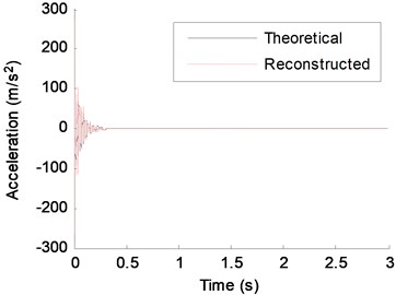
Fig. 18Zoom-in view of a segment (0.2-0.5 s) of Fig. 17
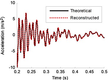
Table 6MAE and RE (%) values in the response reconstruction under different damping levels
Damping level | Error | DOF number | |
2 | 2 | ||
Low damping ratio (, 1e-5) | MAE | 1.61 | 1.61 |
RE | 2.75 | 2.75 | |
High damping ratio (, 1e-4) | MAE | 1.31 | 1.31 |
RE | 5.13 | 5.13 | |
4.2.4. Case 4: Effect of multiple forces
Fig. 19Theoretical response and reconstructed response of DOF-5 from 1-1.5 s (5 % noise)
The feasibility of the proposed method in the presence of multiple forces acting on different degrees of freedom is also investigated. In real life, persistent stochastic excitation is more common than transient excitation. In this case, two random forces , are applied at DOF-1 and DOF-4 persistently, respectively. The reconstructed acceleration response and the theoretical response of DOF-5 from 1 s-1.5 s are shown in Fig. 19. The two time-curves are very close even with 5 % noise, indicating very high reconstruction accuracy of the reconstruction method. In addition, different levels of noise have been also added to the measured signals. MAE and RE under different noise levels are listed in Table 7. Results in Table 7 suggest an overall satisfactory agreement between the reconstructed responses and actual responses and they illustrate that the proposed method is still applicable in the presence of multiple forces acting on different degrees of freedom.
Table 7MAE and RE (%) values in the response reconstruction under different noise levels in Case 4
Noise level (%) | Error | DOF number | Noise level (%) |
2 | 5 | ||
0 | MAE | 1.88 | 0.86 |
RE | 2.85 | 2.51 | |
2 | MAE | 2.35 | 1.32 |
RE | 2.98 | 2.71 | |
5 | MAE | 3.41 | 2.22 |
RE | 3.80 | 3.56 |
4.2.5. Case 5: Two sets of closely spaced modes
In real life, a structure may contain not only one set of closely spaced modes. In this case, two sets of closely spaced modes are assumed here for validation of dynamic response reconstruction. The stiffness coefficients are changed in order to have two sets of closely spaced modes, as listed in Table 8. The Fourier spectra of the response at DOF-1 is plotted in Fig. 20. It is observed that the 2nd and 3rd, 4th and 5th modes are the two sets of closely spaced modes. Thus, we have (2nd and 3rd), (4th and 5th). The acceleration responses of DOF-1, 2, 4 and 6 are assumed known to reconstruct the responses at the rest DOFs. According to Eq. (28), one can obtain:
The reconstructed responses can be obtained easily by Eq. (28). Frequency ranges for each band-pass filter are shown in Table 9. Fig. 21 presents the filtered results of the modal responses at DOF-1. The reconstructed acceleration response and the theoretical response of DOF-3 are shown in Fig. 22. Good agreement between the two signals can be seen from it, which indicates that the proposed method are applicable for the case of a few sets of closely spaced modes.
Table 8Stiffness coefficients of the structure system for Case 5
1 | 1 | 10 | 11 | 7 | 7 | 8 | 8 | 6 | 1 | 2 |
Unit: stiffness-N/m | ||||||||||
Table 9Frequency ranges for each band-pass filter for Case 5
Mode | I | II, III | IV, V | VI |
Natural frequency | 9.77 | 49.62, 56.18 | 82.30, 87.00 | 173.50 |
Passband corner frequency (Hz) | [6-9] | [44-48.5] | [67-77] | [146-162] |
Stopband corner frequency (Hz) | [10.5-13] | [57.5-62] | [90-100] | [174-190] |
Fig. 20Fourier spectra of acceleration response of DOF-1 for Case 5
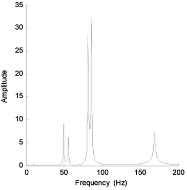
Fig. 21The rest of the modal responses of DOF-1 obtained using the EMD method with intermittency criteria for Case 5
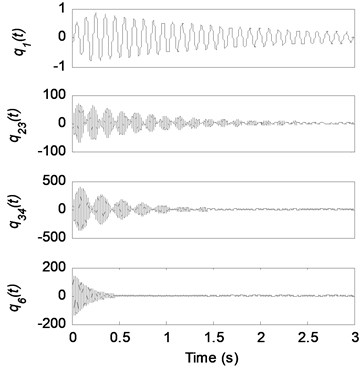
Fig. 22Theoretical response and reconstructed response of DOF-3 for Case 5
5. Conclusions and recommendations
This paper proposes a structural dynamic response reconstruction method for non-proportionally damped system based on the modal superposition method in time domain. The state space method is used to obtain the complex mode shapes. The response reconstruction is based on transforming modal responses from available location to inaccessible locations. The FEM and EMD method with intermittency criteria are the two significant tools of the proposed method. It is suitable for stochastic excitation and transient excitation, such as vibrations induced by ambient wind and earthquakes, the forces are considered to be random, but it is not suitable for periodic excitation which has deterministic frequency. The case of structural system in the presence of closely spaced modes is studied. For this situation, using the proposed method presented in Section 3.2, there is no need to obtain the modal responses of the individual closely spaced modes. A limitation is the number of the known responses must be greater or two times equal than the number of the modes in the set of closely spaced modes. When a structure has a few sets of closely spaced modes, then the number of the known responses must be greater or two times equal than the number of the maximum modes of all the sets of the closely spaced modes. Numerical examples are conducted to validate the accuracy of the proposed methods. Effects of noise in measurements, high damping ratio, multiple forces and two sets of closely spaced modes to the response reconstruction are also investigated in detail. All of the reconstruction results are in good agreement with theoretical predictions.
Current studies assume the finite element model is accurate. Under realistic conditions, the mode shape identified from measurements may introduce uncertainties to the reconstruction results. So the FE model updating is required to be studied on the uncertainties of FE model to the response reconstruction in the future work.
In this paper, only small scale models are investigated, and all the modes are used for reconstructing the responses. For a large scale problem, the higher modes which have extremely small participation factors could be ignored, and this will not decrease the accuracy of the reconstructed responses. Additionally, a real-life experiment should be considered in the future.
References
-
Jardine A. K. S., Lin D., Banjevic D. A review on machinery diagnostics and prognostics implementing condition-based maintenance. Mechanical Systems and Signal Processing, Vol. 20, Issue 7, 2006, p. 1483-1510.
-
Kothamasu R., Huang S. H., VerDuin W. H. System health monitoring and prognostics – a review of current paradigms and practices. The International Journal of Advanced Manufacturing Technology, Vol. 28, Issue 9, 2006, p. 1012-1024.
-
Limongelli M. Optimal location of sensors for reconstruction of seismic responses through spline function interpolation. Earthquake Engineering and Structural Dynamics, Vol. 32, Issue 7, 2003, p. 1055-1074.
-
Kammer D. C. Estimation of structural response using remote sensor locations. Journal of Guidance Control and Dynamics, Vol. 20, Issue 3, 1997, p. 501-508.
-
Jacquelin E., Bennani A., Hamelin P. Force reconstruction: analysis and regularization of a deconvolution problem. Journal of Sound and Vibration, Vol. 265, Issue 1, 2003, p. 81-107.
-
Kerschen G., Worden K., Vakakls A. F., Golinval J. C. Past, present and future of nonlinear system identification in structural dynamics. Mechanical Systems and Signal Processing, Vol. 20, Issue 3, 2006, p. 505-592.
-
Ewins D. J., Liu W. Transmissibility properties of MDOF systems. Proceedings of the 16th International Modal Analysis Conference, Santa Barbara, California, USA, 1998, p. 847-854.
-
Varoto P., McConnell K. Single point vs. multi point acceleration transmissibility concepts in vibration testing. Proceedings of the 16th International Modal Analysis Conference, Santa Barbara, California, USA, 1998, p. 83-90.
-
Ribeiro A., Silva J., Maia N. On the generalisation of the transmissibility concept. Mechanical Systems and Signal Processing, Vol. 14, Issue 1, 2000, p. 29-36.
-
Law S. S., Li J., Ding Y. Structural response reconstruction with transmissibility concept in frequency domain. Mechanical Systems and Signal Processing, Vol. 25, Issue 3, 2010, p. 952-968.
-
Li J., Law S. S. Substructural response reconstruction in wavelet domain. Journal of Applied Mechanics, Vol. 78, Issue 4, 2011, p. 041010.
-
Li J., Law S. S. Damage identification of a target substructure with moving load excitation. Mechanical Systems and Signal Processing, Vol. 30, 2012, p. 78-90.
-
He J., Guan X., Liu Y. Structural response reconstruction based on empirical mode decomposition in time domain. Mechanical Systems and Signal Processing, Vol. 28, 2012, p. 348-366.
-
Yang J. N., Lei Y., Pan S., Huang N. System identification of linear structures based on Hilbert-Huang spectral analysis. Part 1: normal modes. Earthquake Engineering and Structural Dynamics, Vol. 32, Issue 9, 2003, p. 1443-1467.
-
Wan Z., Li S., Huang Q., Wang T. Structural response reconstruction based on the modal superposition method in the presence of closely spaced modes. Mechanical Systems and Signal Processing, Vol. 42, Issue 1-2, 2014, p. 14-30.
-
Djamaa M. C., Ouelaa N., Pezerat C., Guyader J. L. Reconstruction of a distributed force applied on a thin cylindrical shell by an inverse method and spatial filtering. Journal of Sound and Vibration, Vol. 301, Issue 3-5, 2007, p. 560-575.
-
Ambrosino G., Celentano G., Setola R. A spline approach to state reconstruction for optimal active vibration control of flexible systems. Proceedings of the Fourth IEEE Conference on Control Applications, Albany, NY, USA, 1995, p. 896-901.
-
Setola R. A spline-based state reconstruction for active vibration control of a flexible beam. Journal of Sound and Vibration, Vol. 213, Issue 5, 1998, p. 777-790.
-
Adhikari S. Damping Models for Structural Vibration. Ph. D. Thesis, Cambridge University Engineering Department, 2000.
-
Foss K. A. Co-ordinates which uncoupled the equations of motion of damped linear dynamic systems. Journal of Applied Mechanics, Vol. 25, 1958, p. 361-364.
-
Sestieri A., Ibrahim R. Analysis of errors and approximations in the use of modal coordinates. Journal of Sound and Vibration, Vol. 177, Issue 2, 1994, p. 145-157.
-
Huang N. E., et al. The empirical mode decomposition and the Hilbert spectrum for nonlinear and non-stationary time series analysis. Proceedings of the Royal Society of London Series A, Vol. 454, 1998, p. 903-995.
-
Huang N. E., Shen S. S. Hilbert-Huang Transform and its Applications. World Scientific Publishing, 2005.
-
Huang N. E., Shen Z., Long S. R. A new view of nonlinear water waves: The Hilbert Spectrum 1. Annual Review of Fluid Mechanics, Vol. 31, 1999, p. 417-457.
-
Huang K. A nondestructive instrument bridge safety inspection system (NIBSIS) using a transient load. US patent No. 09/210.693, 1988.
-
Liang Z., Lee G. C. Representation of damping matrix. Journal of Engineering Mechanics, Vol. 117, Issue 5, 1991, p. 1005-1019.
About this article

This work was supported by the National Natural Science Foundation of China (No. 51175195).
