Estimation of near fault ground motion based on a hybrid source model and a theoretical Green’s function method

1. Introduction

Due to the increasing number of applications of nonlinear analysis techniques aimed at assessing the structural response and estimating the damage from future seismic events, a credible and complete characterization of ground motion is required for earthquake engineeringanalysis. Engineers usually use a suite of recorded accelerograms from past earthquakes for time-series analysis. They select these accelerograms according to certain criteria. However the use of recorded data for prediction of future ground motions produce some problems. For example in some regions that seismicity is low and therefore the number of recorded motions is not sufficient to consider the variability of earthquake ground motion, engineers have to use records from other regions and scale them to match with the elastic design spectrum prescribed by the adopted seismic code. When the structure is located on a particular soil condition, scaling the spectral amplitude of a signal recorded on a rock site does not provide information on the long duration actually generated [1]. Similarly, earthquake ground motions recorded in regions near to faults are different from those observed in the far-fault regions. In near-fault regions, faulting mechanism, direction of rupture propagation (e.g., forward directivity), and the static deformation of the ground surface (e.g., fling-step) significantly affect ground motions. These specifications also may have serious implications for flexible structures [2]. Scaling the records and matching them with the target elastic design spectrum does not consider the specifications of near-field earthquake ground motion.

As an alternative approach, engineers can simulate realistic synthetic seismograms for engineering purposes rather than using records from past earthquakes [3-5]. Applying simulation techniques, engineers can directly use the synthetic time series, so scaling problems is eliminated. However, these simulation techniques need the definition of a large number of input physical parameters. The accurate values of input parameters rarely can be fixed a priori, and this fact limits the use of simulation proceduresin engineering practices. Because of the uncertainty in input parameters, we have to generate a large number of strong motion scenarios to manage the input values in possible ranges. So, a number of ground motion parameters for each site can be generated and statistically analyzed to provide some insights on the probability distributions of ground-motion values and related statistical estimators. Therefore expanding knowledge about each input parameter can reduce overall uncertainty in a seismic scenario.

The objective of this article is to present the procedure to combine the hybrid slip source model of earthquake scenario source with theoretical-based Green’s function simulation method.We then include the effect of uncertainties of different earthquake source parameters in simulation of near-field events.

2. Theoretical method for simulating near-field strong motions

During the last decade, researchers have proposed various numerical approaches for simulating ground shaking. The three well-known procedures for simulation of ground motion are stochastic procedure based on $\omega$-Square source model, empirical Green’s function, and theoretical-based Green’s function methods [6, 7]. Point source [8] and finite fault [9] techniques are $\omega$-Squared based procedures in which the Fourier’s spectrum of the motion at a site is broken into contributions from earthquake source, path, site and type of motion. The difference between these two procedures is that in the former the causative source of earthquake is modeled as a point source, while in the latter the fault plane is discretized into several equal rectangular elements, each of which is treated as point source. Empirical-based Green’s function method [10, 11] uses the recordings of small events to reproduce large ground motions. Theoretical-based Green’s function method [12] computes the displacement components of ground motion based on Green’s function analytically. We can also find use of above methods in the form of hybrid to reproduce broadband seismogram in engineering problems [13, 14].

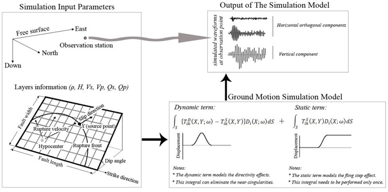
However, there are limited number of consistent procedures to model the specifications of near field earthquakes such as fling step and forward directivity. There is a modified form of Green’s function solution proposed by Hisada and Bielak [15] that considers fling step and forward directivity effects at near-fault sites. In this approach the singularities of the original Green’s functions are eliminated by subtracting and adding the static Green's function in the following form:

where, $U_k$ is the $k$th component of displacement in the Cartesian coordinate system, $Y$ and $X$ are an observation point (i.e. the point location where the simulated ground motion characteristics are monitored) and a source point on the fault plane, respectively, $S$ is the fault plane, $D_i$ is the $i$th component of the fault slip, and $T_{ik}^D$ and $T_{ik}^S$ are the dynamic and static traction Green’s functions of layered half-spaces. The simulation of near-fault ground motions through Eq. (1) is much more efficiently than the original representation theorem [16] which is represented by the total traction Green’s function alone. The original representation theorem requires a lot of CPU time to numerically evaluate the near-singularities of the dynamic Green's function, which show sharp peaks centered at the source point. The first integral of Eq. (1), in which the static Green's function is subtracted from the dynamic function, models the directivity effect. This integral can also eliminate the near-singularities, because the static function includes all the sources of the singularities of the dynamic function. The second integral involves the static Green’s function and models the fling step effect. The near singularities appear only in this integral. The evaluation of this integral necessitates distribution of a set of integration points in the neighborhood of the observation point. However, this integration needs to be performed only once, as the values of the static functions remain invariant for all frequencies. Also in the near field ground motion simulation, in which the source is close to the observation point, it’s needed to compute a lot of Green’s functions. So, the wavenumber integrations of Green’s functions require a lot of CPU time, because the integrands do not converge to zero when the wavenumbers increased [17]. To cope with this problem, Hisada and Bielak [15] used the following wavenumber integrations to evaluate the integral of the first integrand of Eq. (1), since the dynamic Green’s functions are already subtracted by the static Green’s functions:

where $t_{ik}^D$ and $t_{ik}^S$ are the dynamic and static terms of the integrands of the traction Green’s functions, respectively. Since the dynamic integrand converges exactly to the static integrand with increasing wavenumber, the integrand of Eq. (2) attenuates rapidly. A schematic diagram illustrating the simulation process is shown in Fig. 1. References [15, 17] are recommended for researchers who interested in more details. This extended kinematic source method is implemented in the GRFLT12S code by Hisada and Bielak [15]. A number of researchers [18, 19] has recently used this approach and has demonstrated the efficiency of this procedure in simulation of near-field strong ground motion.

Fig. 1Simulation of near field ground motion

3. Hybrid slip model considering uncertainty in source parameters

Advances in understanding the source of past earthquakes led to efforts to estimate future earthquake source properties, and a large amount of work has been done in recent years to estimate the distribution of slip on the fault plane during earthquakes. However, accurate determination of heterogeneous slip on the fault plane before an earthquake is not possibleat the present time. The asperity model and the $k$-square slip modelare two well-known probabilistic approaches for prediction of heterogeneous slip on fault plane. The asperity model first quantified by Somerville et al. [6] using slip distributions of 15 events, and developed by Wang [20] and Wang and Tao [21] by using slip distributions of 29 events. Different relationships between moment magnitude of earthquake and source/asperity parameters is developed based on this model. Herrero and Bernard [22] proposed the $k$-square slip model, in which the slip spectrum decays as $k^{-2}$slip in the wave numbers larger than the corner wave number. Later, Gallovic and Brokesove [23] developed two-dimensional $k$-square slip model.

Recently, the hybrid slip model is presented using combination the asperity and $k$-square models [24, 25]. An example of the hybrid slip model containing two asperities is shown in Fig. 2. To generate the fault model, the moment magnitude of earthquake scenario is at first determined from seismic hazard analysis [26]. Based on this moment magnitude, the fault model parameters (such as the fault dimensions, the number of asperities, the dimensions of asperities, the location of asperities on the fault plane, the average slip on the fault plane, and the average slip on the asperities) are determined by statistical empiricalrelations. The fault plane is divided into a number of subfaults and the deterministic slips are assigned to each subfault (Fig 2(a)). The slip on the fault plane is transferred from spatial domain into wave number domain using two-dimensional Fourier transform. Then k-square slip model is used to generate random slip for wave numbers higher than corner wave number (Eq. (3)):

where $k_{cx}$ and $k_{cy}$ are corner wave numbers along strike and down dip, $\mathrm{\Phi }(k_x,k_y)$ is phase spectrum, $\stackrel{-}{D}$ is the average slip on the fault, $L$ and $W$ are the length and width of fault. Finally, deterministic and random part are superposed in wave number domain and transferred back into spatial domainwith adding noises to deterministicpart of slip distribution (Fig. 2(b)).

Previous studies show that in the case of using the hybrid slip source model and stochastic finite fault simulation technique to generate synthetic accelerograms, the estimated acceleration response spectra is consistent with the recorded response spectra at periods lower than 1.0 sec, but for intermediate and high periods the results are overestimated [27]. This discrepancy may result from the essence of the stochastic finite fault models that tend to overestimate the structural response in long period [28]. To overcome this problem, we use the theoretical-based Green’s function method that models the low frequency motions more precisely. So, we evaluate the efficacy of hybrid slip model for the prediction of motions in longer periods.

Fig. 2An example of the hybrid slip model with two asperities: a) the deterministic part of the slip distribution, b) the resulting hybrid slip

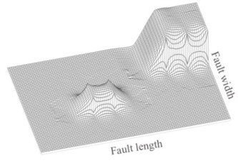
a)

b)

4. Simulation of the 1994 Northridge earthquake

In this section we assume the 1994 Northridge earthquake ($M_W=$6.7) as a future seismic event, considering that no previous studies (as waveform inversion analysis) are available to constrain the source model. We generate the plausible sources by hybrid slip procedure and simulate several possible shaking scenarios. Table 1 shows the relations and their deviations of fault model parameters and location of hypocenter within fault plane.We use the empirical relations proposed by Wang [20] and Wang and Tao [21] in which the uncertainties in both global and local source parameters are considered in fault model simulation.Assuming one up to four different asperities on fault plane [6] and varying hypocenter location within fault plane, one hundred fault models are generated using hybrid slip source model.

Rake angle is assumed variable over the fault plane and is allowed to vary within the range of 55 to 145 degrees [29]. Slip-velocity function is the functional form of slip-velocity with time and its details influence ground motions. In this paper, three different source time functions namely rectangular, triangle and exponential slip-velocity functions [30] are used with multiple time window for each subfault on the simulated ground motion. Rise time is the time period between rupture initiation time and the time of peak moment release rate. This parameteris highly variable on the fault plane. We use the empirical relationship between the value of rise time and the seismic moment of target earthquake, $M_0$, proposed by Somerville et al. [6]:

This equation yields a rise time of 1.01 second for Northridge earthquake with $M_w=$ 6.7. So, we selected rise time of 1.01±1 second with uniform distribution to consider the uncertainty of this parameter. The rupture velocity is defined as the speed at which rupture front propagates on the fault plane and controls the signal duration and contributes to the directivity effect. We assumed the rupture velocity in the narrow range of 0.65–0.85 of the shear-wave velocity ($V_S$) which is inferred with the recorded strong motion data in earthquakes around the world [6]. Two crustal velocity models [29] were employed for rock and soil stations (Table 2). For $V_s<$1500 m/s and $V_s>$1500 m/s, the S-wave quality-factor is assumed as $Q_s=$0.02$V_s$ and $Q_s=$0.1$V_s$, respectively. As well as it is assumed that the P-wave quality-factor is $Q_p=$1.5$Q_s$ [31].

Acceleration time histories during the 1994 Northridge earthquake are numerically simulated by combining the Hisada and Bielak procedure [15] with the hybrid slip source model. We generated the synthesized wave forms up to 2.0 Hz, since this limit of frequency is sufficient to reflect the directivity and fling step effects. Two different rock stations of Santa Susana (SSU) and Simi Valley (U55), and a soil station of Newhall Los Angeles county fire department (NHL) in near-field were used to compare the simulated ground motions with the observed ones.

Fig. 3Comparison the simulated with recorded acceleration response spectra at three near-field stations. The gray lines show the acceleration response spectra of 100 simulated ground motions, the black solid lines show the median of simulated acceleration response spectra and the dashed lines indicate the acceleration response spectra of recorded motions in the 1994 Northridge earthquake

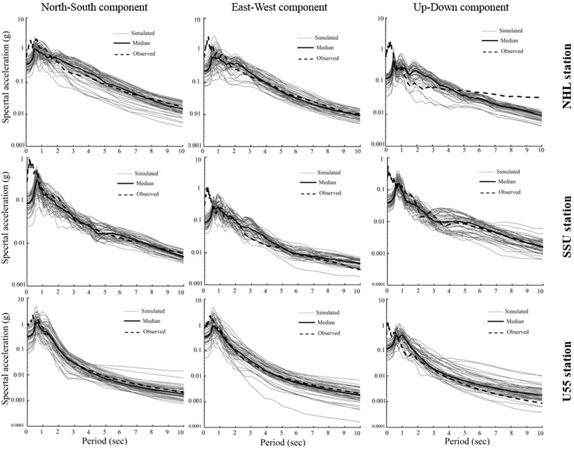
One hundred ground motions were synthesized by using the 100 fault models mentioned above. We discretized the fault planes to 1 km×1 km patches. In each simulation run, the source parameters, namely, the location of hypocenter, rupture velocity, rise time and rake angle were randomly generated from specified distributions and ranges. So, the synthetic database contains 100 earthquake scenarios, all of which are probable. It should be noted that in each simulation run, two horizontal and one vertical component of ground vibration were calculated at each observation point. At each of the three stations, the corresponding acceleration response spectra of the simulated ground motions were worked out with a damping constant of 5 percent. Fig. 3 demonstrates the comparison of the acceleration response spectra corresponding to the simulated and recorded data at three different stations. In this figure, a large scatter compared to the median exists at each station, so the median spectrum actually represents a general level of estimated ground motion.The median acceleration response spectrum is generally consistent with the recorded response spectra for the three stations at periods longer than 1.0 sec. Because of the generation of the synthesized waveforms in narrow band frequencies (0 $\le f\le$ 2 Hz), the mismatch between response spectra extracted by the observed and the synthetic accelerograms is visible. As mentioned before, the results of previous studies show good agreement between recorded ground motions and the simulated ones in frequency domain for periods less than 1.0 sec. Here, in fact we show the efficiency of hybrid slip source model for estimation of near-fault ground motions whose often contain strong coherent dynamic long period pulses and permanent ground displacements and the dynamic motions are dominated by a large long period pulse of motion.

Different source scenarios are examined to find the best fitting between simulated and observed motions recorded at SSU, U55 and NHL stations for different orthogonal directions. Since the best-fitted motions at these stations are from different scenarios of the 100 source scenarios, a systematic search is performed to find the optimum source parameters that provide the best fitting between observed and simulated low-frequency ground motions. We estimate the optimal values of source parameters based on simple additive weighting (SAW) method [32]. Because of its simplicity, SAW is the most popular method inmultiple attribute decision making. In SAW technique, the best alternative, $A^{*}$, can be derived by the following equations:

where $u_i\left(x\right)$ denotes the utility of $i$th alternative, $w_j$ denotes the weight of the $j$th criterion, $r_{ij}=(1/x_{ij})/(1/x_j^{*})$ are normalized values of decision matrix elements. Using this method, we can derive the best alternative of the problem response surface.

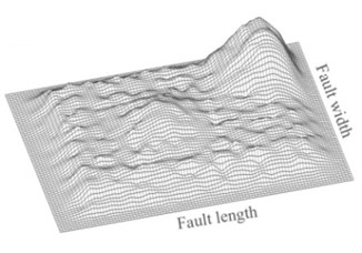
In order to find the optimum source parameters using SAW method, we select peak ground acceleration and acceleration response spectrum as attributes and assign equal weights to the attributes. The optimal fault model obtained via SAW algorithm is shown in Fig. 4. Also the optimal rise time and rupture velocity are 1.43 sec and 2960 m/s respectively which agree with the waveform inversion results [29]. The simulated acceleration time histories from the optimal fault model at the three stations, and their corresponding response spectra are shown in Fig. 5. This figure also provides a comparison in time and frequency domain at NHL, SSU, U55 stations between the simulated motions from the optimal source scenario and the recorded motions in the 1994 Northridge earthquake. Since the simulated data are depicted within the frequency range of 0.0 to 2.0 Hz, recorded acceleration time histories is filtered in this frequency range in order to compare simulated and recorded data in the time domain. Good approximate match of the observed and the simulated waveform, in time and frequency domain at three stations, confirms that the hybrid slip model is an applicable procedure to model seismogenic sources.

Fig. 4Optimal finite fault model for the 1994 Northridge earthquake

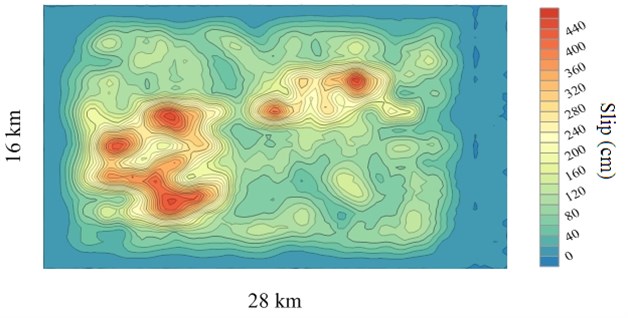
Fig. 5Comparison between the simulated motions from the optimal fault model and the observed motions in the 1994 Northridge earthquake at: a) NHL, b) SSU, c) U55 stations

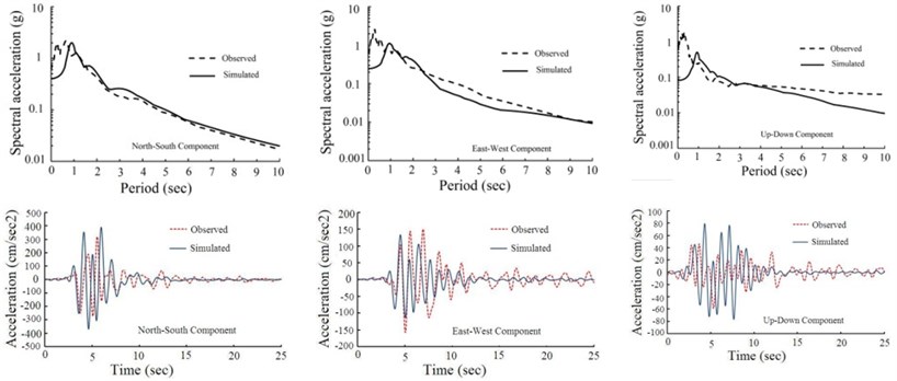
a)

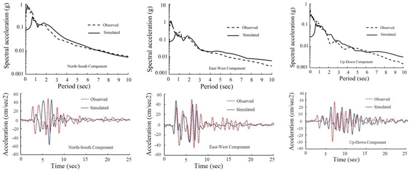
b)

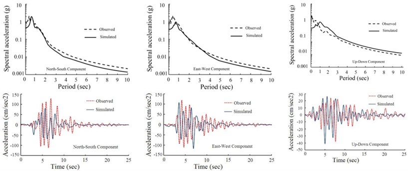
c)

5. Sensitivity of ground motion to source parameters

In this section we perform a sensitivity study to determine which source parameters mostly affect the ground motion. Sensitivity analysis is the study of how the uncertainty in the output of a model can be apportioned to different sources of uncertainty in its inputs [33]. Sensitivity analysis is used to increase understanding of the relationships between input variables and output in a simulation model and to know the relative contribution of each input variable to uncertainty in output of the model. So, the variables that do not contribute much to uncertainty in model output can be fixed at their best estimates, rather than treated as random, in order to simplifying the analysis problem. Also, the variables that cause significant uncertainty in the output can then be the focus of attention to understand them better and reduce uncertainty. There are a large number of approaches to performing a sensitivity analysis, such as scatter plots, regression-based methods, variance-based methods, etc. We used the local sensitivity analysis approach [34] in which the sensitivity of the model output to the model inputs has been examined by varying selected input one-at-a-time around its expected values and observing its effect on the desired model output. In this approach, one parameter is varied a time while the other parameters are kept constant at their nominal values, and this is repeated for each of the other inputs in the same way.

The sensitivity of ground motion to the source parameters has been studied by several authors [1, 23]. However, only few studies attempt to assess how the uncertainties in the different source parameters (especially the fault model and location of hypocenter within fault plane) propagate to near-field ground motion.

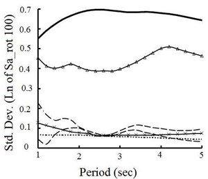
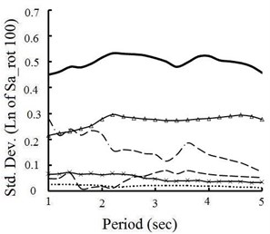
Earthquake intensity measure is an attribute of the strength of an earthquake ground motion and is used to predict earthquake damage and the seismic responses of structures. Studies have shown that the common intensity measures (such as peak ground acceleration) cannot provide an adequate description of the damaging effects of near-fault ground motions which arestrongly influenced by forward directivity and fling step phenomena. Boore [35] proposed the maximum direction (i.e., 100th percentile) value of spectral accelerations computed over all rotation angles for two orthogonal horizontal ground motion components, Sa-rot100, as intensity measure for near-field earthquake ground motions. The effect of uncertainties in source parameters on the variability of Sa-rot100 is investigated in this section.

Fig. 6Variaition of maximum value of spectral response for individually randomized source parameters at: a) 3 km and b) 100 km distances

a)

b)

The impact of source parameters on ground response variability is assessed using Hisada and Bielak [15] model, examining the effect on standard deviation of the maximum direction value of spectral accelerations caused by alternatively varying and fixing different parameters. Fig. 6(a) and 6(b) present fluctuation plots of standard deviation of Sa-rot100 for distances of 3 and 100 km. For generating each spectrum, one of the source parameters is varied while holding the remaining parameters fixed to base case values. These figures show that fault model mostly contribute to variability of ground motion at near- and far-field ground motions. The location of hypocenter within fault plane has strong impact on ground motion variability near fault, but its impact on response variabilitydeclinesas fault-to-site distance increases. Other source parameters (i.e. rake angle, rise time, rupture velocity and slip velocity function) do not contribute significantly on the ground response compared to fault model and hypocenter location, and the sensitivity of them depends on the structural periods of interest. The results show that the increasing knowledge about the source model can significantly reduce the uncertainty in prediction of future earthquake ground motion.

6. Conclusions

In this paper, the theoretical-based Green’s function method of synthesized ground motion is combined with the hybrid slip source model and simple additive weighting method to predict near-field ground motion. Also, we introduce uncertainties of global and local source parameters in the proposed procedure. The proposed procedure is applied to simulate the strong motion of three different near-field stations in the 1994 Northridge earthquake. Good agreement between the synthesized and recordings, in terms of response spectra and time-series, confirms the reliability and ability of these models.

In the hybrid broadband ground motion simulation method, low and high frequency ground motions are simulated by different seismological models, and are then added in the time domain to produce a broadband ground motion. So, utilization of hybrid broadband ground motion simulation method and itscombination with hybrid slip source model can be useful in estimation of near fault ground motion for engineering practices and confirms the reliability of over models in extrapolating procedure. Local sensitivity analysis is performed to investigate the importance of each source parameter. Results show that fault model and location of hypocenter within fault plane are the main important parameters on variability of ground motion.