Abstract
Stochastic analysis of a load moving on a beam is conducted in which the Spectral Stochastic Finite Element Method (SSFEM) is adopted to simulation the uncertainties in the system parameters and excitation forces. Since the dimension of Polynomial Chaos Expansion (PCE) of the beam responses will exponentially grow with the number of K-L components of the system and excitation uncertainties, this limits the application of the SSFEM. A reduced PCE model is proposed in this paper to improve the computational efficiency. The non-Gaussian random variables in the Karhunen-Loéve Expansion (KLE) of the non-Gaussian system parameters are assumed “uncoupled”. Numerical simulations show that the computational effort can significantly be reduced while accurate predictions on the response statistics can still be achieved. Studies on the effect of different level of randomness in the system parameters and excitation forces show that the proposed method has good performance even with a high level of uncertainty.
1. Introduction
The model of “Moving loads on the beam” is widely adopted in simulating engineering problems such as “moving vehicles on bridge deck”, “planes landing on the runway” and “cargos transport by moving overhead crane”, etc. Traditional methods for analyzing the bridge response under moving vehicles can be mainly categorized into two kinds: (1) methods based on modal superposition technique [1, 2]; (2) methods based on finite element method [3, 4].
All the above methods are deterministic approaches in which uncertainties in the bridge structure and the excitation due to moving vehicle are not considered. However, the bridge-vehicle system often exhibits an inherent randomness in the system parameters such as the elastic modulus, mass density, boundary conditions, etc. Furthermore, the interaction forces between the bridge and vehicles are stochastic due to the irregular road surface profile which is usually defined with a power spectral density according to the ISO standard [5]. The samples of the excitation forces are generated from the power spectral density function which will be different from each other. When different samples of the excitation forces are adopted in conventional deterministic analysis, different response samples will be obtained, and this may lead to inaccurate judgment by engineers. In all, the treatment in deterministic analysis only represents an “approximation” of the actual reality in general due to these inherent uncertainties in the structural properties and boundary conditions as well as in the loading process. Stochastic approaches can give a better description on the bridge-vehicle interaction.
The bridge-vehicle interaction problem has been studied considering the uncertainty in the excitation forces with the Monte Carlo Simulation (MCS) method [6], and with stochastic methods in the time domain [7] and in the frequency domain [8]. Others extended the work by introducing Gaussian uncertainties in the system parameters. Fryba et al. [9] performed the stochastic finite element analysis with first-order perturbation to evaluate the variance of the deflection and bending moment of a beam on foundations with uncertain damping and stiffness under a moving force. Dynamic analysis of an Euler-Bernoulli beam excited by a moving oscillator with random mass, velocity and acceleration has been investigated by Muscolino et al. [10] with the improved perturbation approach. Chang et al. [11, 12] studied the dynamic response of an Euler-Bernoulli beam with uncertain parameters such as random mass, stiffness, damping, etc. which is subjected to a moving oscillator/half-car model with random velocity and acceleration. Wu and Law [13] performed dynamic analysis on the bridge-vehicle interaction problem considering Gaussian uncertainties using Karhunen-Loéve expansion. However, the system parameters are always positive in engineering practice, and it is more appropriate to model them with non-Gaussian assumption. Wu and Law [14] later considered the non-Gaussian system parameters in the bridge-vehicle interaction problem where the full dimension of the PCE was adopted in the uncertainty modeling. Liu et al. [15] treated the uncertain system parameters of a bridge-vehicle model as interval variables and perform an interval dynamic analysis on the bridge-vehicle interaction system with these uncertainties.
Though the Spectral Stochastic Finite Element Method (SSFEM) employed by Wu and Law [14] can improve the accuracy of analysis with perturbation technique when the level of uncertainty increases, the SSFEM suffers from the curse of exponentially increased dimension in the Polynomial Chaos Expansion for the solution when the required number of the Karhunen-Loéve (K-L) components for both the system parameters and excitation is large [16]. In the dynamic analysis of a bridge structure, when the excitation force includes high frequency random fluctuations, e.g. vehicle excitation arising from road surface roughness or the ground motion excitation due to an earthquake, a relative large number of K-L components maybe included, e.g. larger than 100 components as shown in the numerical simulation of this paper. It is noted that in the PCE for a random process, the number of K-L components adopted is usually not larger than twenty [17]. This drawback limits the application of the SSFEM in the case with relatively simple excitation forces.
In this paper, a reduced PCE model is proposed to replace the “full” PCE model in SSFEM. A non-Gaussian stochastic process model including high frequency random fluctuations can be represented efficiently with the proposed reduced model. Accurate response statistics of the beam under the moving loads can also be predicted using the proposed stochastic finite element method.
2. System equation of motion with uncertainty
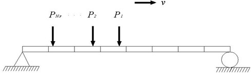
A two-dimensional simply supported Euler-Bernoulli beam with multiple loads moving on top is shown in Fig. 1. The mass per unit length , elastic modulus and damping of the beam structure are assumed as non-Gaussian random processes, with mean value , , and standard deviation , , , respectively. The random part of the these parameters, denoted as , , , can be obtained by subtracting the mean value from the random variable.
The equation of motion of the structure with random material properties and randomness in the excitations can then be written as:
where is the cross-sectional area, is the moment of inertia of the beam and denotes the random dimension. is the number of the moving forces. Employing the Hermitian cubic interpolation shape functions and with the assumption of Rayleigh damping for the structure, the equation of motion of the beam can be rewritten in matrix form as:
where , , are the stochastic mass, damping and stiffness matrices of the beam model with , , , respectively. , , , , , are the deterministic and random components of the system mass, damping and stiffness matrices respectively, and they can be obtained by assembling the corresponding elemental matrices as:
where and are respectively the shape function matrix and strain-displacement matrix for each element. is the length of beam element. is the stochastic force vector applied on the beam structure with . , and are the stochastic nodal displacement, velocity and acceleration vectors of the structure respectively with . is a × location matrix of the moving forces as shown in Eq. (4), where is the number of degree-of-freedom of the beam structure after considering the boundary condition. We have:
where the shape function vector can be written in the global coordinate as:
and is the location of the th force on the th element at time with . The two coefficients and of the Rayleigh damping:
are assumed constant, and they can be obtained from the mean values of the first two modal frequencies and damping ratios. The stochastic displacement of the beam at position and time has the following relationship with the stochastic nodal displacement as:
where and is the shape function of the beam structure. is a 1× vector with zero entries except at the th beam element on which the force is located.
Fig. 1The beam-moving load system
3. Karhunen-Loéve expansion
3.1. Theory [18]
Let be a second-order random process and denote the expected value of . The covariance function of is bounded, symmetric and positive definite and has the following spectral decomposition:
where and are the eigenvalues and the eigenvectors of the covariance function, respectively. They can be proved to be solution of the following integral equation:
Due to symmetry and the positive definiteness of the covariance kernel, the eigenfunctions are orthogonal and they form a complete set representing the covariance function. The eigenvectors can then be normalized according to the following criterion:
where is the Kronecker delta. The random process can then be written as:
where is a group of uncorrelated random variables. As a special case, when is a Gaussian random process, is a set of standard Gaussian random variables with the following orthogonal properties:
where denotes the expectation value.
4. Polynomial Chaos expansion
4.1. Theory [19]
For an element from a set in the space spanned by the orthogonal basis, it has been proved that can be written in the following form as:
where are the Hermite polynomials of , ,…, , and 1.0, 1.0. are the generalized Fourier coefficients with (0, 1,…, ) and . The series in Eq. (13) can be refined along the random dimension either by increasing the total number of random variables or the maximum order of polynomials included in the Polynomial Chaos (PC) expansion. The first refinement takes into account higher frequency random fluctuations of the underlying stochastic process, while the second refinement captures strong nonlinear dependence of the solution of this stochastic process [20].
The polynomials are orthogonal satisfying the relationship:
where denotes the inner product and the value of can be calculated analytically [19].
The generalized Fourier coefficients in Eq. (13) can be evaluated from:
4.2. Polynomial Chaos coefficients
Numerous approaches have been proposed to obtain the coefficients in the PCE model for a random process. Field et al. [21] proposed two methods with Monte Carlo simulation and numerical integration, respectively, to evaluate the coefficients. Non-intrusive method and Intrusive method were adopted by Reagan et al [22] for the analysis. The method using Latin Hypercube sampling and Fitting Regression model [23] will be introduced as follows due to its high efficiency and great accuracy, and it will be adopted in this paper to evaluate the coefficients in a one-dimensional PCE in the proposed reduced PCE model.
For a one-dimensional problem, i.e. in Eq. (13) equals to unity, consider the PCE truncated at the th level:
where , 0, 1, 2,…, , are the regression coefficients, and is the error of the model equation. Functions , ,…, are the th one-dimensional Hermite polynomials of .
It is noted that Eq. (16) can be regarded as a linear regression model. To evaluate the coefficients , sample values, e.g. ~, should be drawn from the standard random variable . With these sample values, the matrix form can be formulated as:
where , , and:
and to are the sample values drawn from . Vector includes the error terms. The sample values of ( 1, 2,…, ) in Eq. (17) can be obtained from the Cumulative Density Function (CDF) of the random variables.
Using the least-squares method, the regression coefficients can be calculated as:
The fitted model and the residuals are:
5. Modeling with non-Gaussian uncertainties
5.1. The reduced PCE model
The KLE of a non-Gaussian process results in a set of deterministic coefficients multiplied by the corresponding uncorrelated non-Gaussian random variables . In the PCE of a non-Gaussian process, these uncorrelated non-Gaussian random variables are projected on the Polynomial Chaos basis. The dimension of PCE, denoted as ,to represent the stochastic response of a beam structure is determined according to the following [20]:
where is the maximum order of the Polynomial Chaos in PCE; is the number of K-L components required in the representation of the response which depends on the number of K-L components adopted in the representations of excitation forces and system parameters. For example, if the randomness in elastic modulus, mass density and excitation forces are independent and the Rayleigh damping is assumed, then . Variables , , are the number of K-L components in the KLE of the Gaussian distributed elastic modulus, mass density and the excitation forces, respectively.
When a large number of K-L components is required inthe KLE of the excitation force, an extremely large number of Polynomial Chaos will be included in the PCE of the non-Gaussian random responses according to Eq. (20), and this leads to computation problem due to the limited capability of computer. This drawback limits the application of the SSFEM in the case with relatively simple excitation.
For the case with complex excitation forces, a reduced PCE model is proposed to avoid the curse of dimensionity of PCE in the response representation. The uncorrelated random variables in the KLE of the non-Gaussian random processes are assumed to be “uncoupled”. The spaces spanned by these “uncoupled” random variables are assumed to be mutually orthogonal, which results in keeping the terms of in Eq. (13) and eliminating the terms of in the new reduced model. For example, when 2 and 2, Eq. (13) has the following form:
and in the new reduced model, the terms , and are eliminated while other terms are retained. It is noted that the variance of a non-Gaussian system parameter is derived from the following equation:
Since the variance of terms retained are larger than those of the eliminated ones when they are of the same order [19], e.g. the variance of and are equal to 6 and 2, respectively, when the total number of the random variables increases, the summation of the variance of terms retained will be much larger than that of the eliminated ones. Therefore, the accuracy in the variance representation in Eq. (22) may still be maintained.
The reduced PCE approach on a non-Gaussian random process is implemented as follows: After the decomposition of a non-Gaussian random process along the dimension and using the finite element method and KLE respectively, each uncorrelated random variable , which is assumed as “uncoupled” in this reduced PCE model, can be expanded as shown in Eq. (16) with a one-dimensional Polynomial Chaos. The dimension of PCE, , required in a reduced PCE of order for the stochastic response becomes:
It is noted from Eqs. (20) and (23) that the dimension of PCE under this “uncoupled” assumption is significantly reduced compared with that in the “full” PCE. This allows the proposed algorithm to include a large number of K-L components in the PCE of the excitation force or the system parameters, with a trade off in the accuracy.
5.2. Modeling of the non-Gaussian system
5.2.1. The system matrices
According to the system equation of motion as described in Section 2, the KLE is applied to the elastic modulus according to Eq. (11) as:
where is the number of K-L components. are the normalized non-Gaussian random variables. Then:
The stochastic system stiffness matrix ) can then be expressed as:
where can be assembled from . Let and 1.0, we have:
According to the reduced PCE for the non-Gaussian random process introduced in Section 5.1, the system matrices can be summarized as follows:
The stochastic system mass matrix can similarly be expressed as:
Since the Rayleigh damping matrix is a linear combination of the system mass and stiffness matrices according to Eq. (6), the damping matrix can also be written as:
where , , . , and are deterministic coefficients corresponding to the th K-L component and th order of the Polynomial Chaos for the elastic modulus, mass density and damping, respectively. Variable is the order of Polynomial Chaos adopted, , and are the number of the K-L components adopted for the elastic modulus, mass density and damping, respectively. , and are the number of terms of the Polynomial Chaos in the reduced PCE for the elastic modulus, mass density and damping, respectively. According to the assumption of the reduced PCE, the relationship between the number of K-L components and the number of Polynomials for the PCE of the three system parameters are:
5.2.2. The excitation forces
The stochastic excitation forces can be expanded similarly according to Eq. (28) as:
where and is the deterministic coefficient corresponding to ; , and are the number of K-L components, the order of Polynomial Chaos and the dimension of the reduced PCE for the excitation force vector, respectively.
5.2.3. The responses
The nodal displacement vector of the system with non-Gaussian property can be represented by the reduced PCE after truncation as:
where is the dimension of the reduced PCE related to the order of the Polynomial Chaos and the number of K-L components for the stochastic displacement vector with and .
Taking the first and second derivatives of Eq. (33) with respect to , the stochastic velocity and acceleration vectors can be obtained respectively as:
where and .
5.2.4. The dynamic equation of equilibrium
Substituting Eqs. (28) to (30) and (32) to (35) into Eq. (2), and taking inner product of both sides of Eq. (2) with respect to and employing the orthogonal property of Polynomial Chaos in Eq. (14), we have:
Let:
Eq. (36) can be written in matrix form as:
The values of inner product of polynomial chaos are constants and they can be obtained analytically [19].
5.3. Response statistics
Eq. (37) can be solved by employing the Newmark- method to obtain the deterministic coefficients in the reduced PCE for the responses, and the first two response statistics of the stochastic nodal displacement vector can be evaluated as:
where the subscript “” denotes the random nodal displacement vector of the beam structure. The stochastic displacement of the beam structure at position and time can be derived according to Eqs. (7) and (38) as:
The mean and variance of the stochastic displacement at position and time can be respectively obtained as:
where the subscript “” denotes the random displacement of the beam. The mean value and variance of the stochastic velocity and acceleration at position and time can also be obtained by substituting the first and second derivatives and obtained from Eq. (37) into Eq. (40). Samples of the stochastic displacement of the beam structure at position and time can be generated from Eq. (39) with any available sampling techniques, e.g. the Latin Hypercube sampling [24], to simulate the Gaussian random variables in the Polynomial Chaos . The probabilistic density function of the stochastic displacement of the beam structure at position and time can then be obtained from Eq. (39) after the coefficients are calculated.
6. Numerical simulations
The following properties of the beam model are adopted in the numerical simulation: length of beam 40 m; cross-sectional area 4.8 m2; second moment of inertia of cross-section 2.5498 m4; damping ratio 0.02 for all modes; elastic modulus and the mass density are assumed as random variables with mean value 5×10¹⁰ N/m2 and 2.5×10³ kg/m3respectively and with a coefficient of variation denoted as and , respectively. The mean value of the first five natural frequencies of the beam are 3.9, 15.6, 35.1, 62.5 and 97.6 Hz. Rayleigh damping is assumed.
The random time-varying moving forces are generated with the following mean values:
and with different Coefficients of Variation () at each time instant. The two loads are moving at a specific speed four meters apart as a group. It should be noted that although only two random forces are considered in the simulation, more forces can be included according to Eq. (1).
The relative error between the statistics of the calculated and reference responses are calculated as:
Since the system parameters are always positive in engineering practice, both the system parameters and the excitation forces are assumed as lognormal random processes in this study. To describe the uncertainty in the system parameters for the beam structure, covariance kernels for the stochastic system parameters have to be defined. The finite element model of beam is assumed to have eight Euler-Bernoulli beam elements of 5 m long each. In this simulation, the following exponential auto-covariance function is adopted as the covariance function for the stochastic system parameters:
where is the standard deviation of system parameter or . Expression denotes the positive distance between two points in a spatial domain of interest. is the correlation length. The positive distance between two points in a spatial domain of interest is set equal to 0.5 m unless it is stated otherwise and is set as unity for both the elastic modulus and mass density in the following study. It should be noted that the covariance function for the two system parameters can be totally different with different values of and . The sampling rate for all the simulations is 200 Hz. Results from the proposed algorithm is compared with those from the Monte Carlo Simulation on 10000 samples for verification.
6.1. Coefficients in the one-dimensional Polynomial Chaos expansion
According to the proposed method, the one-dimensional PCE for each uncoupled non-Gaussian random variable should be performed. A numerical study is conducted to compare the efficiency and accuracy of different existing techniques, such as, the Latin Hypercube sampling and the Fitting Regression model proposed by Choi et al. [23]. Considering the two functions and including the normal random variable with a zero mean value and unit standard deviation as:
The coefficients in the one-dimensional PCE of the two functions are calculated with different existing techniques and with different order of PC up to four. The relative error and the time required in the calculation of coefficients of PCE using MCS method [21] with 10000 samples, the Latin Hypercube Sampling (LHS) method [22] with 300 samples, and Fitting Regression Model (FRM) method [23] using 300 samples respectively are shown in Table 1. The programme runs on a computer with Intel Core 2, Quad CPU 2.40 Hz and 8 GB RAM. Results show that the Fitting Regression Model method has both high efficiency and accuracy comparing with the other two methods especially for random variables which can be approximated as Polynomial functions of Gaussian random variables. Therefore, this method will be adopted in the following study to calculate the coefficients in the one-dimensional PCE in the reduced PCE model.
Table 1Relative Error (%) in coefficients of one dimensional PCE calculated from three methods
Methods | MCS | LHS | FRM | MCS | LHS | FRM |
0.07 | 0.14 | 0 | 0.01 | 0.06 | 0.03 | |
0.04 | 0.98 | 0 | 0 | 0.29 | 0.29 | |
0.09 | 1.84 | 0 | 0.05 | 0.61 | 0.24 | |
0.23 | 2.75 | 0 | 0.08 | 0.80 | 0.67 | |
0.02 | 2.81 | 0 | 0.08 | 0.80 | 0.25 | |
Time (s) | 35.34 | 0.17 | 0.14 | 33.07 | 0.14 | 0.11 |
6.2. Effect of the level of randomness in system parameters
Different levels of randomness in the system parameters, i.e. different and are investigated. Different orders of Polynomial Chaos are adopted to represent the lognormal random processes of system parameters. To highlight the effect of the level of randomness in system parameters on the accuracy of the non-Gaussian model, the two excitation forces are assumed as deterministic ( 0%) in this Section as defined in Eqs. (41) and (42).
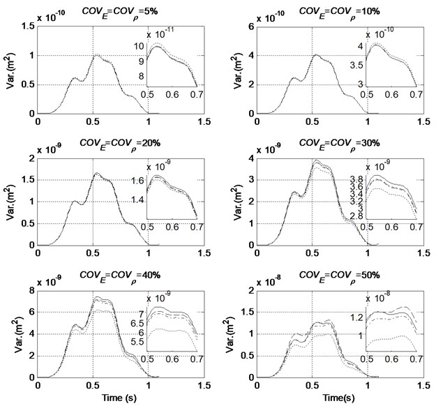
The mean value and variance of the mid-span displacement of the beam structure calculated with the proposed method under different order of PC and the MCS are compared in Figs. 2 and 3, respectively. The detail informations from 0.5 s to 0.7 s are also demonstrated to achieve a better understanding of the results.
The relative errors of the results compared with those from the MCS according to Eq. (43) are listed in Table 2.
Results show that the calculated mean values for all the cases are very accurate and the relative error increases slightly with the increase of level of randomness in system parameters. The order of PC adopted has little effect on the accuracy of calculated mean value in general. For the variance of the mid-span displacement, the use of a low order of PC such as an order of 2, can achieve a high accuracy as noted in Table 2 when the and are small and below 0.2. The results from large COV values can, however, be improved with the use of 3rd and 4th order PC, and the result from a 4th-order representation is better that that from a 3rd-order representation. Large error exists in the calculated variance when only a 2nd-order PCE is adopted for the cases with and larger than 0.2.
Table 2Relative error (%) in mid-span displacement statistics due to different level of PC representation when COVF= 0 %
0 % | Order of PC | 5 % | 10 % | 20 % | 30 % | 40 % | 50 % |
Mean value | 2 | 0.01 | 0.02 | 0.03 | 0.06 | 0.31 | 0.84 |
3 | 0.01 | 0.02 | 0.06 | 0.20 | 0.56 | 1.34 | |
4 | 0.01 | 0.02 | 0.06 | 0.22 | 0.68 | 1.85 | |
Variance | 2 | 0.63 | 1.51 | 2.58 | 8.31 | 14.85 | 21.66 |
3 | 0.06 | 0.14 | 1.51 | 3.27 | 4.77 | 5.00 | |
4 | 0.08 | 0.11 | 1.36 | 2.88 | 3.01 | 8.11 | |
Fig. 2Comparison of the mean mid-span displacement with different order of PC (COVF= 0 %, — MCS, ----- Order 2, –·– Order 3, – – Order 4)
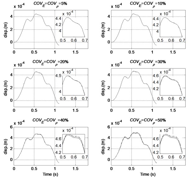
Fig. 3Comparison of variance of mid-span displacement with different order of PC (COVF= 0 %, — MCS, ----- Order 2, –·– Order 3, – – Order 4)
Another observation noted in Table 2 is that for a very large and , e.g. larger than 0.4, the mean and variance from a 3rd-order representation are better that that from a 4th-order representation. This phenomenon can be explained as follows: the error in the coefficient calculation from the one-dimensional polynomial chaos expansion will be amplified by the K-L components of the random processes, and it will propagate into the reduced PCE model causing larger errors. It may be concluded that when more coefficients in the one-dimensional PCE are included in the calculation with higher order Polynomial Chaos, the computation error will be amplified and accumulated affecting the accuracy of the calculated response statistics.
Via the comparison of response statistics with the MCS method in Table 2, the accuracy of the proposed method is proved. The proposed method also has good efficiency, for example, in the case when 20 %, 10 min is required for 10000 runs of MCS to obtain the response statistics and only 15 s is needed for the proposed method.
6.3. Effect of the distance of interest
It is noted that a refined distance between two points in a spatial domain of interest will increase the number of K-L components in the PCE of a non-Gaussian system parameter. According to Section 5.1, to increase the total number of K-L components in the reduced PCE can improve the accuracy of variance representation of the non-Gaussian parameter. Although the number of the KLE increases in this reduced PCE, yet the total number of Polynomial Chaos adopted under the assumption of “uncoupled” is much smaller than that in a “full” PCE.
Fig. 4Comparison of variance of mid-span displacement with different distance of interest (Order of PC = 3, COVF= 0 %, — MCS, -*- 0.5 m, ----- 1 m, –·– 2.5 m, – – 5 m)
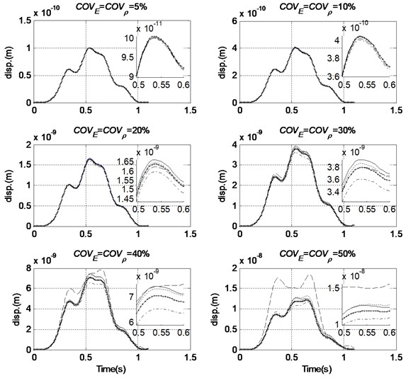
A numerical study is carried out on the moving load on beam system with 0 % and the order of PCE equals to three in this sub-section to show the effect of the distance of interest on the accuracy of the predicted variance of the response. A comparison between the predicted variance of response using MCS and the reduced PCE method with different distance of interest are shown in Fig. 4, and the corresponding relative errors are shown in Table 3. The detail informations from 0.5 s to 0.6 s are also demonstrated in Fig. 4 to achieve a better understanding of the results.
Results show that when the level of randomness in the system parameters is not large, e.g. 0.2, with a relative large distance of interest 5.0 m, that is 1/8 of the total length of the beam, the relative error in the predicted variances of the response is less than 4 % indicating a good accuracy. When the level of randomness increase, with 5.0 m, larger error exists in the predicted variance of response. By decreasing the distance of interest, the relative error in the predicted variance of the response can be significantly reduced. For example, when the level of randomness in the system parameters has a 0.5, and the distance of interest is decreased from 5.0 m to 1.0 m, the relative error in the predicted variance of response reduced from 57.3 % to 3.68 % according to results in Table 3. The relative error in the predicted variance of response decreases with smaller distance between two points of interest. It is noted from Table 3 that such reduction can be achieved favourably when 1.0 m. Due to the “uncoupled” assumption made in the proposed reduced PCE model, the relative error in the predicted variance of response is not linearly decreasing with the distance of interest.
Table 3Relative error (%) in variance of mid-span displacement due to different distance of interest when COVF= 0 % and Order of PC = 3
0 % | Distance of interest (m) | 5 % | 10 % | 20 % | 30 % | 40 % | 50 % |
Variance | 5 | 0.23 | 0.64 | 1.94 | 3.09 | 11.9 | 57.3 |
2.5 | 0.32 | 1.03 | 3.79 | 7.38 | 10.1 | 10.7 | |
1 | 0.15 | 0.33 | 1.15 | 1.97 | 2.04 | 3.68 | |
0.5 | 0.06 | 0.14 | 1.51 | 3.27 | 4.77 | 5.00 | |
6.4. Effect of the level of randomness in excitation
Investigations on the effect of the level of randomness in excitation is similarly conducted with 20 % in this section. Different levels of randomness of the lognormal distributed excitation forces are adopted with different order in the Polynomial Chaos.
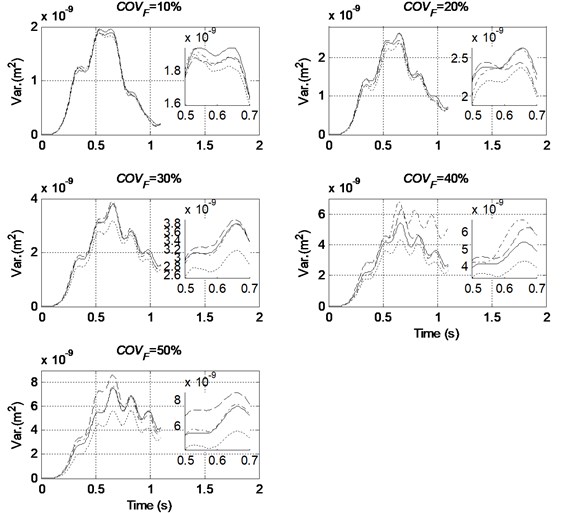
The mean and variance of the mid-span displacement of the beam structure obtained using the proposed method with different order of PCE and from the MCS are compared in Figs. 5 and 6, respectively. The detail informations from 0.5 s to 0.7 s are also demonstrated to achieve a better understanding of the results.The relative errors according to Eq. (43) from both methods are listed in Table 4.
Table 4Relative error (%) in mid-span displacement statistics due to different level of PC representation when COVE=COVρ= 20 %
20 % | Order of PC | 10 % | 20 % | 30 % | 40 % | 50 % |
Mean value | 2 | 1.81 | 1.90 | 1.99 | 2.11 | 2.24 |
3 | 1.79 | 1.83 | 1.84 | 1.87 | 1.91 | |
4 | 1.79 | 1.83 | 1.83 | 1.80 | 1.88 | |
Variance | 2 | 4.23 | 11.2 | 14.0 | 17.8 | 23.1 |
3 | 3.35 | 4.44 | 3.93 | 4.83 | 5.21 | |
4 | 3.59 | 6.90 | 3.82 | 12.5 | 16.2 | |
Results show that the order of Polynomial Chaos has little effect on the accuracy of the mean mid-span displacement. When the are equal or larger than 0.2, a relatively large error exists in the calculated variance from a 2nd-order representation. When the becomes large, e.g. at 0.4 or 0.5, a 3rd-order representation has better performance than a 4th-order representation. The reason for this phenomenon has been explained in the last paragraph in Section 6.2.
Fig. 5Comparison of mean mid-span displacement with different level of randomness in excitation and different order of PC used (COVE=COVρ= 20 %, — MCS, ----- Order 2, –·– Order 3, – – Order 4)
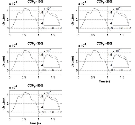
Fig. 6Comparison of variance of mid-span displacement with different level of randomness in excitation and different order of PC used (COVE=COVρ= 20 %, — MCS, ----- Order 2, –·– Order 3, – – Order 4)
It may be concluded that when a system with the coefficients of variation of both the system parameters and excitation forces smaller than 0.2, a 2nd-order representation of the Polynomial Chaos should be sufficient to obtain accurate response statistics of the system. In other cases with larger coefficients of variation, a 3rd-order representation of Polynomial Chaos is recommended. When the coefficient of variation of the excitation forces attains a large value of 0.5, the response statistics of the non-Gaussian model with a reduced PCE could still maintain a good accuracy.
7. Conclusions
A reduced PCE model is proposed in this paper to represent the non-Gaussian system parameters in a stochastic moving load on beam system. With the “uncoupled” assumption on the uncorrelated non-Gaussian random variables in the KLE of the non-Gaussian system parameters, the curse of dimensionality in a full PCE model can be alleviated with acceptable predictions on the response statistics of the beam. Numerical simulations with the proposed method and from the MCS show good agreement in the result for cases with different level of uncertainties in the excitation and system parameters and different order of Polynomial Chaos used. The following conclusions can be drawn:
1) The SSFEM with the proposed reduced PCE model can achieve good accuracy in the mean and variance predictions even when the and are as large as 0.5. When and are smaller or equal to 0.2, the proposed approach has good accuracy even with large uncertainties in the excitation forces. The relative errors in the first two response statistics of the beam responses increase with an increase in the level of randomness in both the system parameters and excitation forces.
2) When the level of randomness in the system parameters is 0.2, with a distance of interest equal to 1/8 total length of the beam, the relative error in the predicted variances of the response are less than 4 %; when the level of randomness increases to 50 %, an error in the predicted variances of the response up to 57.3 % will occur. The relative error in the predicted variances of the response can be significantly reduced to below 5 % when the distance of interest is decreased.
3) For a system with the coefficients of variation of both the system parameters and excitation forces smaller than 0.2, a 2nd-order representation of the Polynomial Chaos should be sufficient to obtain accurate response statistics of the beam structure. In other cases of larger coefficients of variation, a 3rd-order representation of Polynomial Chaos is recommended.
References
-
Marchesiello S., Fasana A., Garibaldi L., Piombo B. A. D. Dynamic of multi-span continuous straight bridges subject to multi-degrees of freedom moving vehicle excitation. Journal of Sound Vibration, Vol. 224, Issue 3, 1999, p. 541-561.
-
Zhu X. Q., Law S. S. Dynamic behavior of orthotropic rectangular plates under moving loads. Journal of Engineering Mechanics, Vol. 129, Issue 1, 2003, p. 79-87.
-
Henchi K., Fafard M., Talbot M., Dhatt G. An efficient algorithm for dynamic analysis of bridges under moving vehicles using a coupled modal and physical components approach. Journal of Sound Vibration, Vol. 212, Issue 4, 1998, p. 663-683.
-
Lee S. Y., Yhim S. S. Dynamic behavior of long-span box girder bridges subjected to moving loads: Numerical analysis and experimental verification. International Journal of Solids and Structures, Vol. 42, Issues 18-19, 2005, p. 5021-5035.
-
ISO 8606:1995(E). Mechanical Vibration – Road Surface Profiles – Reporting of Measured Data. 1995.
-
Sasidhar M. N. V., Talukdar S. Nonstationary response of bridge due to eccentrically moving vehicle at variable velocity. Advances in Structural Engineering, Vol. 6, Issue 4, 2003, p. 309-324.
-
Seetapan P., Chucheepsakul S. Dynamic responses of a two-span beam subjected to high speed 2DOF sprung vehicles. International Journal of Structural Stability and Dynamics, Vol. 6, Issue 3, 2006, p. 413-430.
-
Da Silva J. G. S. Dynamical performance of highway bridge decks with irregular pavement surface. Computers and Structures,Vol. 82, Issues 11-12, 2004, p. 871-881.
-
Fryba L., Nakagiri S., Yoshikawa N. Stochastic finite elements for beam on a random foundation with uncertain damping under a moving force. Journal of Sound Vibration, Vol.163, Issue 1, 2003, p. 31-45.
-
Muscolino G., Benfratello S., Sidoti A. Dynamics analysis of distributed parameter system subject to a moving oscillator with random mass, velocity and acceleration. Probabilistic Engineering Mechanics, Vol. 17, 2002, p. 63-72.
-
Chang T. P., Lin G. L., Chang E. Vibration analysis of a beam with an internal hinge subject to a random moving oscillator. International Journal of Solids and Structures,Vol. 43, 2006, p. 6398-6412.
-
Chang T. P., Liu M. F., O H. W. Vibration analysis of a uniform beam traversed by a moving vehicle with random mass and random velocity. Structural Engineering and Mechanics, Vol. 31, Issue 6, 2009, p. 737-749.
-
Wu S. Q., Law S. S. Dynamic analysis of bridge-vehicle system with uncertainties based on the finite element model. Probabilistic Engineering Mechanics, Vol. 25, 2010, p. 425-432.
-
Wu S. Q., Law S. S. Dynamic analysis of bridge with non-Gaussian uncertainties under a moving vehicle. Probabilistic Engineering Mechanics, Vol. 26, 2011, p. 281-293.
-
Liu N., Gao W., Song C., Zhang N., Pi Y. Interval dynamic response analysis of vehicle-bridge interaction system with uncertainty. Journal of Sound Vibration, Vol. 332, 2013, p. 3218-3231.
-
Stefanou G. The stochastic finite element method: past, present and future. Computer Methods in Applied Mechanics and Engineering, Vol. 198, 2009, p. 1031-1051.
-
Eiermann M., Ernst O. G., Ullmann E. Computational aspects of the stochastic finite element method. Computing and Visualization in Science, Vol. 10, Issue 1, 2007, p. 3-15.
-
Schenk C. A., Schuëller G. I. Uncertainty Assessment of Large Finite Element Systems. Springer-Verlag, Berlin Heidelberg, 2005.
-
Ghanem R., Spanos P. D. Stochastic Finite Elements: A Spectral Approach. Springer-Verlag, New York, 1991.
-
Ghanem R. Stochastic finite elements with multiple random non-Gaussian properties. Journal of Engineering Mechanics-ASCE, Vol. 125, Issue 1, 1999, p. 26-40.
-
Field R. V. Numerical methods to estimate the coefficients of the polynomial chaos expansion. 15th ACSE Engineering Mechanics Conference, Columbia University, New York, 2002.
-
Reagan M. T., Najm H. N., Ghanem R., Knio O. M. Uncertainty quantification in reacting-flow simulations through non-intrusive spectral projection. Combustion and Flame, Vol. 132, 2005, p. 545-555.
-
Choi S. K., Grandhi R. V., Canfield R. A., Pettit C. L. Polynomial chaos expansion with latin hypercube sampling for estimating response variability. AIAA Journal, Vol. 42, Issue 6, 2004, p. 1191-1198.
-
Florian A. An efficient sampling scheme: updated latin hypercube sampling. Probabilistic Engineering Mechanics, Vol. 7, 1992, p. 123-130.
About this article

The research work was supported by a research grant from the National Natural Science Foundation of China (No. 11402052), the Natural Science Foundation of Jiangsu province (No. BK20140616), the Specialized Research Fund for the Doctoral Program of Higher Education of China (20130092120039) and the Priority Academic Program Development of Jiangsu Higher Education Institutions (PAPD).
