Stochastic stability and moment Lyapunov exponent for co-dimension two bifurcation system with a bounded noise

Li, Shenghong; Wu, Jiancheng

Journal of Vibroengineering

Browse Journal

Submit article

Published: 30 December 2015

Check for updates

Stochastic stability and moment Lyapunov exponent for co-dimension two bifurcation system with a bounded noise

Shenghong Li¹

Jiancheng Wu²

^{1, 2}School of Mathematics and Physics, Jiangsu university of Science and Technology, Zhenjiang 212003, Jiangsu Province, China

²State Key Lab of Mechanics and Control for Mechanical Structures, College of Aerospace Engineering, Nanjing University of Aeronautics and Astronautics, 29 Yudao Street, Nanjing 210014, China

Corresponding Author:

Shenghong Li

Cite the article Download PDF

Downloads 1266

Abstract

In this paper, the $p$ th moment Lyapunov exponent of a co-dimension two bifurcation system that is parametrically excited by a real noise is investigated. By a linear stochastic transformation, the eigenvalue problem of moment Lyapunov exponent is obtained. Then through perturbation method, we deduce the joint probability density function of the phase processes and its eigenvalue problem, which is solved by a Fourier cosine series expansion. Thus, an infinite matrix yields and whose leading eigenvalue is the second order of the asymptotic expansion of the moment Lyapunov exponent. Because of the complexity of elements in matrix $A$ , the eigenvalues of the low order sub-matrices of $A$ are obtained by the truncation of $n$ and the convergence of the eigenvalue sequence is numerically illustrated. Finally, the effects of the system and noise parameters on the moment Lyapunov exponent are discussed.

1. Introduction

The moment Lyapunov exponent that describes the $p$ th moment stability of stochastic dynamic system, is defined as:

1

Λ (p, x_{0}) = \underset{t \to \infty}{l i m} \frac{1}{t} l o g E [{‖x (t, x_{0})‖}^{p}],

where $x (t, x_{0})$ is a solution to a random dynamical system and $E [\cdot]$ denotes expected value. If $Λ (p, x_{0}) < 0$ , by definition, $E [{‖x (t, x_{0})‖}^{p}] \to 0$ as $t \to \infty$ , which represents that the $p$ th moment of the stochastic system is stable. The relation between moment stability and almost-sure stability for an un-damped linear oscillator under real noise excitation was found firstly by Molcanov [1]. Later, the results were extended to an arbitrary $d$ -dimensional system by Arnold in Ref. [2], meanwhile, the rigorous definition of the moment Lyapunov exponent was firstly defined and the following results were obtained. Under some conditions, the limit in Eq. (3) exists and is independent of the initial value $x_{0}$ . So the moment Lyapunov exponent can be written as $Λ (p)$ , which is a convex analytic function of $p \in R$ . In addition, the maximal Lyapunov exponent is a derivative of moment Lyapunov exponent at $p =$ 0, i.e.:

2

λ = {\frac{\partial Λ (p)}{\partial p}|}_{p = 0} = \underset{t \to \infty}{l i m} \frac{1}{t} l o g ‖x (t, x_{0})‖ .

Then, Aronld investigated the linear stochastic systems excited by the real noise and white noise, and given a series of results of the moment Lyapunov exponent respectively in [3, 4]. Thus, the stochastic problem of linear system was resolved completely.

However, it is extremely difficult to investigate the stochastic stability of a nonlinear dynamical system except for several very special cases, especially for moment stability. So far, almost all the investigations on the moment Lyapunov exponents are confined to the approximate analytical methods. For a two dimensional stochastic system, L. Arnold [5] firstly applied a perturbation method to perform the asymptotic expansions of the $p$ th moment Lyapunov exponents on a small noise intensity and a small value of $p .$ Using the same method, Namachchivaya [6] obtained the small $p$ th moment Lyapunov exponent for a system with two coupled oscillators that is excited by a real noise. For a linear conservative system with a white noise, Khasminskii and Moshchuk [7] proved that the finite $p$ th moment Lyapunov exponent and the stability index can respectively be expressed only as the asymptotic expansions of small noise intensity. On the basis of the theorem given in [7], for the same system and random excitation as [6], Namachchivaya and Roessel [8] obtained the asymptotic expansion of the finite $p$ th moment Lyapunov exponent. For the two dimensional system that was driven by the real noise and the bounded noise excitations respectively, Xie [9-10] implemented the weak noise expansions of the finite $p$ th moment Lyapunov exponent, the maximal Lyapunov exponent and the stability index through the same procedure. In recent years, this topic is still a hotspot for the researchers in the field of random dynamical system. The stability properties of a Van der Pol-Duffing oscillator with a real noise was investigated by Liu [11]. Due to the complexity of approximate analytical methods, Higham [12] gave the numerical simulation of moment Lyapunov exponent in stochastic differential equations. Then, the moment Lyapunov exponent and the stochastic stability of a double-beam system under the compressive axial loading and moving narrow bands was studied by Kozic [13]. Shenghong Li [14, 15] presented the result of the moment Lyapunov exponent for a three dimensional stochastic system. For a binary airfoil system driven by non-Gaussian colored noise, DL Hu [16] obtained its moment Lyapunov exponent.

In this paper, the $p$ th moment Lyapunov exponent of a co-dimension two bifurcation system that is parametrically excited by a real noise is investigated. For the same system, the maximal Lyapunov exponent was investigated by Li [17, 18]. In Section 2, the studied dynamical system is introduced and the eigenvalue problem of moment Lyapunov exponent is obtained. In Section 3, through a perturbation method, the probability density functions of differential operator about $ε^{0}$ , $ε^{1}$ and $ε^{2}$ are solved respectively. In Section 4, via an expansion of orthogonal Fourier series, the eigenvalue problem of the differential operator leads to the eigenvalue problem for an infinite matrix, whose leading eigenvalue is the moment Lyapunov exponent. The numerical results are presented in Section 5 and a conclusion is given in Section 6.

2. Formulation

Consider a typical deterministic co-dimension two bifurcation system that is on a three-dimension central manifold and possesses one zero-eigenvalue and a pair of pure imaginary eigenvalues [19], i.e.:

3

\dot{r} = μ_{1} r + a_{1} r z + (a_{2} r^{3} + a_{3} r^{2} z) + O ({|r, z|}^{4}),

\dot{z} = μ_{2} z + (b_{1} r^{2} + b_{2} z^{2}) + (b_{3} r^{2} z + b_{4} z^{3}) + O ({|r, z|}^{4}),

\dot{Θ} = ω + O ({|r, z|}^{2}),

where $μ_{1}$ and $μ_{2}$ are unfolding parameters, $a_{1}$ , $a_{2}$ , $a_{3}$ , $b_{1}$ , $b_{2}$ , $b_{3}$ and $ω$ is real constants. This normalized form arises in the classic fluid dynamic stability study of coquette flow.

According to Oseledec multiplication ergodic theorem in the theory of random dynamical system, both invariant manifold of the nonlinear system and the relevant invariant subspace of its linearized system are tangent at the equilibrium point, thus the almost asymptotic stabilities for the two systems at the equilibrium point are the same. Therefore, in order to study the stability for a nonlinear stochastic system at the equilibrium point, it is sufficient we only investigate the stochastic stability of its corresponding linearized system within the vicinity of the equilibrium point by the results.

Via the transformation of $r = (x_{1}^{2} + x_{2}^{2})^{1 / 2}$ , $z = x_{3}$ , $Θ = a r c t a n (x_{1} / x_{2})$ in the vicinity of equilibrium point $x' = (x_{1}, x_{2}, x_{3}) = (0, 0, 0)$ , the linearization of the original system Eq. (3), which is subjected to a stochastic parametric perturbation, is the following as:

4

\{\begin{array}{l} \dot{x} = A_{0} x - ε^{2} A_{1} x + ε c o s (ξ (t)) B x, \\ d ξ (t) = μ d t + σ \circ d W (t), \end{array}

where:

A_{0} = [\begin{matrix} 0 & ω & 0 \\ - ω & 0 & 0 \\ 0 & 0 & 0 \end{matrix}], A_{1} = [\begin{matrix} δ_{1} & 0 & 0 \\ 0 & δ_{1} & 0 \\ 0 & 0 & δ_{2} \end{matrix}], B = [\begin{array}{l} b_{11} & b_{12} & b_{13} \\ b_{21} & b_{22} & b_{23} \\ b_{31} & b_{32} & b_{33} \end{array}] .

The symbol ‘ $\circ$ ’ indicates that the equations within Eq. (4) are Stratonovich stochastic differential equations, $μ$ and $σ$ are real constants, $W (t)$ is a unit Wiener process and the bifurcation parameters $μ_{1}$ , $μ_{2}$ are rescaled such that $μ_{1} = - ε δ_{1}$ , $μ_{2} = - ε δ_{2}$ .

The following spherical polar transformation from $(x_{1}, x_{2}, x_{3})$ to $(ρ, θ, ϕ)$ :

5

x_{1} = a c o s θ s i n ϕ, x_{2} = a c o s θ c o s ϕ, x_{3} = a s i n θ, ρ = l n a, P = a^{p},

ϕ (t) = ω t + φ (t), θ \in [- \frac{π}{2}, \frac{π}{2}], ϕ, φ \in [0, 2 π],

yields a set of equations of the arguments of $ρ$ , $θ$ , $ϕ$ and the noise process $ξ (t)$ , i.e.:

6

d P = [ε c o s (ξ) p P ρ_{1} + ε^{2} p P ρ_{2}] d t,

d θ = [ε c o s (ξ) θ_{1} + ε^{2} θ_{2}] d t,

d ϕ = [ω + ε c o s (ξ) ϕ_{1}] d t,

d ξ = μ d t + σ \circ d W (t),

where:

ρ_{1} = \frac{1}{2} (f_{12} + f_{31}) s i n 2 θ + f_{11} c o s^{2} θ + f_{32} s i n^{2} θ,

ρ_{2} = - δ_{1} c o s^{2} θ - δ_{2} s i n^{2} θ,

θ_{1} = \frac{1}{2} (f_{32} - f_{11}) s i n 2 θ + (f_{31} c o s^{2} θ - f_{12}) s i n^{2} θ,

θ_{2} = \frac{1}{2} (δ_{1} - δ_{2}) s i n 2 θ,

ϕ_{1} = f_{21} + f_{22} t a n θ,

f_{11} = \frac{1}{2} (k_{1} + k_{2} c o s 2 ϕ + k_{3} s i n 2 ϕ),

f_{12} = b_{13} s i n ϕ + b_{23} c o s ϕ,

f_{21} = \frac{1}{2} (k_{4} + k_{3} c o s 2 ϕ - k_{2} s i n 2 ϕ),

f_{22} = b_{13} c o s ϕ - b_{23} s i n ϕ,

f_{31} = b_{31} s i n ϕ + b_{32} c o s ϕ, f_{32} = b_{33},

k_{1} = b_{22} + b_{11}, k_{2} = b_{22} - b_{11},

k_{3} = b_{12} + b_{21}, k_{4} = b_{12} - b_{21} .

For the norm process $P$ , a reversible linear stochastic transformation is introduced, i.e.:

7

S = T (θ, ϕ, ξ) P, P = T^{- 1} (θ, ϕ, ξ) S, - \frac{π}{2} \leq θ \leq \frac{π}{2}, 0 \leq ϕ \leq 2 π, 0 < ξ < 2 π,

where the function $T (θ, ϕ, ξ)$ is a scalar function of the phase processes $(θ, ϕ, ξ)$ . Thus the equation for the new norm process $S$ is obtained through lemma:

8

d S = P \{μ \frac{\partial T}{\partial ξ} + \frac{1}{2} σ^{2} \frac{\partial^{2} T}{\partial ξ^{2}} + ω \frac{\partial T}{\partial ϕ} + ε (p ρ_{1} T + θ_{1} \frac{\partial T}{\partial θ} + ϕ_{1} \frac{\partial T}{\partial ϕ}) c o s (ξ)

+ ε^{2} (p ρ_{2} T + θ_{2} \frac{\partial T}{\partial θ})\} d t + σ \frac{\partial T}{\partial ξ} P d W .

Since $T (θ, ϕ, ξ)$ is bounded and non-singular, then both $P$ and $S$ have the same stability. Therefore, $T (θ, ϕ, ξ)$ is selected such that the drift term of Eq. (11) is independent of the phase processes $θ$ , $ϕ$ and $ξ$ , i.e.:

9

d S = Λ (p) S d t + σ \frac{\partial T}{\partial ξ} T^{- 1} (θ, ϕ, ξ) S d W .

Comparing between Eq. (8) and Eq. (9) yields a fact that $T (θ, ϕ, ξ)$ is presented by the following equation:

10

Λ (p) T = μ \frac{\partial T}{\partial ξ} + \frac{1}{2} σ^{2} \frac{\partial^{2} T}{\partial ξ^{2}} + ω \frac{\partial T}{\partial ϕ} + ε (p ρ_{1} T + θ_{1} \frac{\partial T}{\partial θ} + ϕ_{1} \frac{\partial T}{\partial ϕ}) c o s (ξ)

+ ε^{2} (p ρ_{2} T + θ_{2} \frac{\partial T}{\partial θ}) .

The above equation is written as:

11

L_{ε} (p) T (θ, ϕ, ξ) = Λ (p) T (θ, ϕ, ξ),

where:

12

L_{ε} (p) = L_{0} (p) + ε L_{1} (p) + ε^{2} L_{2} (p),

L_{0} (p) = μ \frac{\partial}{\partial ξ} + \frac{σ^{2}}{2} \frac{\partial^{2}}{\partial ξ^{2}} + ω \frac{\partial}{\partial ϕ},

L_{1} (p) = (θ_{1} \frac{\partial}{\partial θ} + ϕ_{1} \frac{\partial}{\partial ϕ} + p ρ_{1}) c o s (ξ),

L_{2} (p) = θ_{2} \frac{\partial}{\partial θ} + p ρ_{2} .

And its corresponding adjoint operator is:

13

L_{0}^{*} = - μ \frac{\partial}{\partial ξ} + \frac{σ^{2}}{2} \frac{\partial^{2}}{\partial ξ^{2}} - ω \frac{\partial}{\partial ϕ},

L_{1}^{*} = - [θ_{1} \frac{\partial}{\partial θ} + ϕ_{1} \frac{\partial}{\partial ϕ} + p ρ_{1}] c o s (ξ),

L_{2}^{*} = - θ_{2} \frac{\partial}{\partial θ} + p ρ_{2} .

We can see that Eq. (11) defines an eigenvalue problem with the second-order differential operator, in which, $Λ (p)$ is the eigenvalue and $T (θ, ϕ, ξ)$ is the eigenfunction. Based on Eq. (11), one can easily find that this eigenvalue is the $p$ th moment Lyapunov exponent of system Eq. (4).

Consider the operator $L_{ε} (p)$ and its adjoint operator $L_{ε}^{*} (p)$ , according to the facts shown by Arnold [3, 4], $Λ (p)$ is an isolated simple eigenvalue of $L_{ε} (p)$ with non-negative eigenfunction $T (θ, ϕ, ξ)$ and $‖T (θ, ϕ, ξ)‖ = 1.$ For $L_{ε}^{*} (p),$ $T^{*} (θ, ϕ, ξ)$ is the unique eigenfunction corresponding to $Λ (p)$ with the property of $⟨T (θ, ϕ, ξ), T^{*} (θ, ϕ, ξ)⟩ = 1$ , i.e.:

14

L_{ε} (p) T (θ, ϕ, ξ) = Λ (p) T (θ, ϕ, ξ),

L_{ε}^{*} (p) T^{*} (θ, ϕ, ξ) = Λ (p) T^{*} (θ, ϕ, ξ),

⟨T (θ, ϕ, ξ), T^{*} (θ, ϕ, ξ)⟩ = 1, \forall p \in R .

3. Asymptotic analysis

Because it is practically impossible that the expression of $Λ (p)$ is solved by Eq. (14), perturbation method is applied here. The following asymptotic expansions $Λ (p)$ and $T (θ, ϕ, ξ)$ are assumed in advance, i.e.:

15

Λ (p) = Λ_{0} (p) + ε Λ_{1} (p) + ε^{2} Λ_{2} (p) + \dots + ε^{n} Λ_{n} (p) + \dots,

T (θ, ϕ, ξ) = T_{0} (θ, ϕ, ξ) + ε T_{1} (θ, ϕ, ξ) + ε^{2} T_{2} (θ, ϕ, ξ) + \dots + ε^{n} T_{n} (θ, ϕ, ξ) + \dots .

Substituting Eq. (15) into Eq. (14) and equating the terms of the equal powers of $ε$ , then the following recursion equations are obtained:

16

ε^{0} : L_{0} (p) T_{0} (θ, ϕ, ξ) = Λ_{0} (p) T_{0} (θ, ϕ, ξ),

ε^{1} : L_{0} (p) T_{1} (θ, ϕ, ξ) + L_{1} (p) T_{0} (θ, ϕ, ξ) = Λ_{0} (p) T_{1} (θ, ϕ, ξ) + Λ_{1} (p) T_{0} (θ, ϕ, ξ),

ε^{2} : L_{0} (p) T_{2} (θ, ϕ, ξ) + L_{1} (p) T_{1} (θ, ϕ, ξ) + L_{2} (p) T_{0} (θ, ϕ, ξ) = Λ_{0} (p) T_{2} (θ, ϕ, ξ)

+ Λ_{1} (p) T_{1} (θ, ϕ, ξ) + Λ_{2} (p) T_{0} (θ, ϕ, ξ) .

3.1. $ε^{0}$ order perturbation

According to Eq. (16), the zero order perturbation equation is equavelant to:

17

L_{0} (p) T_{0} (θ, ϕ, ξ) = Λ_{0} (p) T_{0} (θ, ϕ, ξ),

i.e.:

18

\frac{σ^{2}}{2} \frac{\partial^{2} T_{0}}{\partial ξ^{2}} + μ \frac{\partial T_{0}}{\partial ξ} + ω \frac{\partial T_{0}}{\partial ϕ} = Λ_{0} (p) T_{0} .

In order to make the problem tractable, we assume $θ$ , $ϕ$ and $ξ$ are mutually independent. Applying the method of variable separation, i.e. $T_{0} (θ, ϕ, ξ) = F_{0} (θ) Φ_{0} (ϕ) H_{0} (ξ)$ , and dividing both sides of Eq. (18) by $Φ_{0} (ϕ) H_{0} (ξ)$ , we obtain:

19

\frac{σ^{2}}{2} \frac{{\ddot{H}}_{0} (ξ)}{H_{0} (ξ)} + μ \frac{{\dot{H}}_{0} (ξ)}{H_{0} (ξ)} - Λ_{0} = - ω \frac{{\dot{Φ}}_{0} (ϕ)}{Φ_{0} (ϕ)} = k .

Solving the equation for $Φ_{0}$ yields $Φ_{0} (ϕ) = k e^{- \frac{c}{ω} ϕ}$ , where $k$ and $c$ are constants. Since $Φ_{0} (ϕ)$ is a periodic function of $ϕ$ , we obtain $c = 0$ . Hence $Φ_{0} (ϕ)$ can be chosen as 1. On the basis of the property of moment Lyapunov exponent, we know $Λ (0) = 0$ , which is substituted into Eq. (15), then leads to that $Λ_{0} (0) = 0$ . Because the left side of Eq. (18) does not include $p$ , $Λ_{0} (0) = 0$ yields $Λ_{0} (p) = 0$ . Thus the equation for $H_{0} (ξ)$ becomes:

20

\frac{σ^{2}}{2} \frac{{\ddot{H}}_{0} (ξ)}{H_{0} (ξ)} + μ \frac{{\dot{H}}_{0} (ξ)}{H_{0} (ξ)} = 0 .

We easily obtain:

21

H_{0} (ξ) = C_{0} + C_{1} e x p (- \frac{2 μ}{σ^{2}}) .

Since $H (ξ)$ is bounded, $C_{1} = 0$ is required. So $H (ξ)$ is a constant, we choose $H (ξ) = 1$ .

Thus, we obtain:

22

T_{0} (θ, ϕ, ξ) = F_{0} (θ), θ \in [- \frac{π}{2}, \frac{π}{2}], ϕ \in [0, 2 π], ξ \in [0, 2 π] .

It is the joint probability density function of the phase processes $(θ, ϕ, ξ)$ .

The corresponding adjoint differential equation of Eq. (17) is the following:

23

μ \frac{\partial}{\partial ξ} T_{0}^{*} - \frac{σ^{2}}{2} \frac{\partial^{2}}{\partial ξ^{2}} T_{0}^{*} - ω \frac{\partial}{\partial ϕ} T_{0}^{*} = 0 .

Also $T_{0}^{*} (θ, ϕ, ξ) = F_{0}^{*} (θ) G_{0}^{*} (ϕ) H_{0}^{*} (ξ)$ , Eq. (23) becomes:

24

\frac{σ^{2}}{2} \frac{{\ddot{H}}_{0}^{*} (ξ)}{H_{0}^{*} (ξ)} - μ \frac{{\dot{H}}_{0}^{*} (ξ)}{H_{0}^{*} (ξ)} = ω \frac{{\dot{Φ}}_{0}^{*} (θ)}{Φ_{0}^{*} (θ)} = κ .

Solving the above equation, we obtain $Φ_{0}^{*} (ϕ) = c_{1} e^{κ / ω}$ . Where $κ$ and $c_{1}$ are constants. Because $Φ_{0} (ϕ)$ is a periodic function of $ϕ$ , then $κ = 0$ , and $Φ_{0}^{*} (ϕ)$ is selected:

Φ_{0}^{*} (ϕ) = \frac{1}{2 π}, ϕ \in [0, 2 π],

which represents the probability density function of a uniformly distributed random variable $ϕ \in [0, 2 π]$ .

Therefore, Eq. (24) is simplified as:

25

\frac{σ^{2}}{2} \frac{{\ddot{H}}_{0}^{*} (ξ)}{H_{0}^{*} (ξ)} - μ \frac{{\dot{H}}_{0}^{*} (ξ)}{H_{0}^{*} (ξ)} = 0 .

The solution of Eq. (25) is $H_{0}^{*} (ξ) = B_{0} + B_{1} e x p (2 μ / σ^{2})$

Since $H^{*} (ξ)$ is bounded, it is required that $B_{1} = 0$ . $ξ (t)$ is the angle of triangular function, and cosine is the periodic function with $2 π$ , so we can choose $H^{*} (ξ) = 1 / 2 π$ , $ξ \in [0, 2 π]$ . Thus:

26

T_{0}^{*} (θ, ϕ, ξ) = \frac{1}{4 π^{2}} F_{0}^{*} (θ), θ \in [- \frac{π}{2}, \frac{π}{2}], ϕ \in [0, 2 π], ξ \in [0, 2 π],

which is the joint probability density of the independent random variables $(θ, ϕ, ξ)$ .

3.2. $ε^{1}$ order perturbation

From Eq. (16), the first order perturbation is the following:

27

L_{0} (p) T_{1} (θ, ϕ, ξ) + L_{1} (p) T_{0} (θ, ϕ, ξ) = Λ_{0} (p) T_{1} (θ, ϕ, ξ) + Λ_{1} (p) T_{0} (θ, ϕ, ξ) .

Substituting $Λ_{0} (p) = 0$ and $T_{0} (θ, ϕ, ξ) = F_{0} (θ)$ into Eq. (27) results as follows:

28

L_{0} (p) T_{1} (θ, ϕ, ξ) = Λ_{1} (p) T_{0} (θ, ϕ, ξ) - L_{1} (p) T_{0} (θ, ϕ, ξ) .

The solvability condition of Eq. (28) is:

29

⟨Λ_{1} (p) T_{0} (θ, ϕ, ξ) - L_{1} (p) T_{0} (θ, ϕ, ξ), T_{0}^{*}⟩ = 0,

where $T_{0}^{*}$ is shown in Eq. (26), $⟨\cdot, \cdot⟩$ denotes the inner product that is defined as follows:

⟨S_{1}, S_{2}⟩ = \int_{0}^{2 π} d ϕ \int_{- π / 2}^{π / 2} d θ \int_{0}^{2 π} S_{1} (θ, ϕ, ξ) S_{2} (θ, ϕ, ξ) d ξ .

Solving Eq. (29) obtains that the first order term of the moment Lyapunov exponent, i.e.:

30

Λ_{1} (p) = ⟨L_{1} (p) T_{0} (θ, ϕ, ξ), T_{0}^{*}⟩ .

Again $T_{0} (θ, ϕ, ξ) = F_{0} (θ)$ , so by calculating it is obtained that:

31

L_{1} (p) T_{0} (θ, ϕ, ξ) = c o s (ξ) [θ_{1} F_{0}^{'} (θ) + p ρ_{1} F_{0} (θ)] .

And $T_{0}^{*} (θ, ϕ, ξ) = F_{0}^{*} (θ) / 4 π^{2}$ , Eq. (31) is rewritten as:

32

Λ_{1} (p) = \frac{1}{4 π^{2}} ⟨\cos (ξ) [θ_{1} F_{0}^{'} (θ) + p ρ_{1} F_{0} (θ)], F_{0}^{*} (θ)⟩ .

Integrating Eq. (32) for $ξ$ from 0 to $2 π$ , it is obtained that $Λ_{1} (p) = 0$ .

Hence, Eq. (27) reduces to:

33

L_{0} (p) T_{1} (θ, ϕ, ξ) = - L_{1} (p) T_{0} (θ, ϕ, ξ),

i.e.:

34

(μ \frac{\partial}{\partial ξ} + \frac{σ^{2}}{2} \frac{\partial^{2}}{\partial ξ^{2}} + ω \frac{\partial}{\partial ϕ}) T_{1} (θ, ϕ, ξ) = - c o s (ξ) [θ_{1} F_{0}^{'} (θ) + p ρ_{1} F_{0} (θ)] .

For the convenience to write, let $F (θ, ϕ) = θ_{1} F_{0}^{'} (θ) + p ρ_{1} F_{0} (θ)$ .

In order to solve the measure $T_{1} (θ, ϕ, ξ)$ , we introduce an auxiliary time $t'$ in Eq. (34) and make it become as:

35

(\frac{\partial}{\partial t^{'}} + \frac{σ^{2}}{2} \frac{\partial^{2}}{\partial ξ^{2}} + μ \frac{\partial}{\partial ξ} + ω \frac{\partial}{\partial ϕ}) T_{1} (θ, ϕ, ξ, t^{'}) = c o s (ξ (t)) F (θ, ϕ) .

Applying the linear transformation $t' = ψ + s$ , $ϕ = ω (ψ + s)$ , then Eq. (35) is:

36

(\frac{\partial}{\partial s} + \frac{σ^{2}}{2} \frac{\partial^{2}}{\partial ξ^{2}} + μ \frac{\partial}{\partial ξ}) T_{1} (θ, ψ, ξ, s) = c o s (ξ (t)) F (θ, ω (ψ + s)) .

According to Duhamel’s principle [20], the solution for Eq. (36) is given by:

37

T_{1} (θ, ψ, ξ, s) = \int_{0}^{s} f (θ, ψ, ξ, s; r) d r,

where $f (θ, ψ, ξ, s; r)$ is the solution of the following homogeneous equations:

38

(\frac{\partial}{\partial s} + \frac{σ^{2}}{2} \frac{\partial^{2}}{\partial ξ^{2}} + μ \frac{\partial}{\partial ξ}) f (θ, ψ, ξ, s; r) = 0, s > r,

f (θ, ψ, ξ, r; r) = c o s (ξ (t)) F (θ, ω (ψ + s)), s = r .

In order to solve Eq. (38), the following equations are considered:

39

(\frac{\partial}{\partial s} + \frac{σ^{2}}{2} \frac{\partial^{2}}{\partial ξ^{2}} + μ \frac{\partial}{\partial ξ}) P (ξ, s; z, t) = 0, s < t,

P (ξ, s; z, t) = \underset{s \to t}{l i m} P (ξ, s; z, t) = δ (z - ξ) .

Eq. (39) are the Kolmogorov’s backward equations for the transition probability function $P (ξ, s; z, t)$ , which is the probability density function of random variable $z (t)$ conditioned on $ξ (s)$ , $t > s$ . The transition probability function with Eq. (4) is given:

40

P (ξ, s; z, t) = \frac{1}{\sqrt{2 π (t - s)} σ} e x p \{- \frac{z - [ξ + μ (t - s)]}{σ^{2} (t - s)}\} .

By Eq. (38) and Eq. (39), the solution for Eq. (38) is given by:

41

f (θ, ψ, ξ, s; r) = F (θ, ω (ψ + r)) \int_{- \infty}^{+ \infty} E \{c o s [z (r)]\} P (ξ, s; z, t) d z,

where:

42

E \{c o s [z (r)]\} = \int_{- \infty}^{+ \infty} \cos [z (r)] P (ξ, s; z, r) d z = c o s [ξ - μ (r - s)] e x p \{- \frac{1}{2} σ^{2} (r - s)\} .

After substituting Eq. (41) and Eq. (42) into Eq. (37) and via some calculation, $T_{1} (θ, ψ, ξ, s)$ is solved:

43

T_{1} (θ, ψ, ξ, s) = e x p [- \frac{1}{2} σ^{2} (t - s)] {c o s (ξ) \int_{0}^{s} F (θ, ω (ψ + r)) c o s [μ (r - s)] d r

+ s i n (ξ) \int_{0}^{s} F (θ, ω (ψ + r)) \sin [μ (r - s)] d r} .

Meanwhile, the solution $T_{1} (θ, ψ, ξ)$ in Eq. (34) is obtained by inserting $ϕ = ω (ψ + s)$ into Eq. (43) and calculating the limit $s \to - \infty$ .

3.3. $ε^{2}$ order perturbation

According to Eq. (16), the second order perturbation is rewritten as:

44

L_{0}^{} T_{2} = Λ_{2} T_{0} - L_{1}^{} T_{1} - L_{2}^{} T_{0} = Λ_{2} T_{0} - c o s (ξ) (θ_{1} \frac{\partial}{\partial θ} + ϕ_{1} {\frac{\partial}{\partial ϕ}}_{1} + p ρ_{1}) T_{1}

- θ_{2} F_{0}^{'} (θ) - p ρ_{2} F_{0} (θ) .

The solvability condition of Eq. (44) is:

45

\frac{1}{4 π^{2}} \int_{0}^{2 π} d ϕ \int_{- \frac{π}{2}}^{\frac{π}{2}} d θ \int_{0}^{2 π} [Λ_{2} T_{0} - c o s (ξ) (θ_{1} \frac{\partial}{\partial θ} + ϕ_{1} {\frac{\partial}{\partial ϕ}}_{1} + p ρ_{1}) T_{1}

- θ_{2} F_{0}^{'} (θ) - p ρ_{2} F_{0} (θ)] \cdot F_{0}^{*} (θ) d ξ = 0 .

Via an integral for $ϕ$ on $[0, 2 π]$ and the massive calculations, Eq. (45) can be sorted into:

46

\int_{- π / 2}^{π / 2} \{[L (p) - Λ_{2} (p)] F_{0} (θ)\} F_{0}^{*} (θ) d θ = 0,

L (p) = \frac{1}{2} σ^{2} (θ) \frac{d^{2}}{d θ^{2}} + [μ (θ) + p \hat{μ} (θ)] \frac{d}{d θ} + [p q (θ) + \frac{1}{2} p^{2} \hat{q} (θ)],

σ^{2} (θ) = \frac{1}{32} (2 α_{1}^{2} σ_{3} - α_{2} σ_{2}) s i n^{2} (2 θ)

+ [\frac{1}{2} α_{4} - α_{5} c o s^{2} (θ) + \frac{1}{2} α_{3} c o s^{4} (θ)] σ_{1} [c o s (2 θ) - c o s^{4} (θ)],

μ (θ) = \frac{1}{64} [9 α_{6} μ_{1} - (3 α_{5} + 16 α_{4}) σ_{1} + 4 (α_{2} σ_{2} - (k_{1}^{2} - k_{1}) σ_{3}) + 32 Δ^{-}] s i n (2 θ)

+ \frac{1}{64} [2 α_{1}^{2} σ_{3} + 6 (α_{5} σ_{1} + α_{4} μ_{1}) - (α_{5} σ_{1} + α_{2} σ_{2}) + 4 α_{4} σ_{1}] s i n (4 θ)

+ \frac{1}{64} (α_{6} μ_{1} - 3 α_{5} σ_{1}) s i n (6 θ) + \frac{1}{128} α_{3} σ_{1} s i n (8 θ) + \frac{1}{4} α_{4} σ_{1} t a n (θ),

\hat{μ} (θ) = \frac{1}{128} [2 (α_{2} σ_{2} + 5 α_{5} σ_{1}) - 8 (k_{1}^{2} - 4 b_{33}^{2}) σ_{3}

- (11 b_{32}^{2} - 16 b_{23}^{2} - 6 b_{31}^{2} + 16 b_{13}^{2}) σ_{1}] s i n (2 θ)

- \frac{1}{64} [2 (α_{1}^{2} σ_{3} + b_{32}^{2} α_{2} σ_{1}) + 4 (α_{4} + α_{5} + b_{23}^{2}) σ_{1} - α_{2} σ_{2}] s i n (4 θ)

+ \frac{1}{128} (2 α_{3} + 2 b_{31}^{2} + b_{32}^{2}) σ_{1} s i n (6 θ),

q (θ) = \frac{1}{2} [α_{6} μ_{1} - (α_{4} + α_{5}) σ_{1}]

+ \frac{1}{4} [α_{1}^{2} σ_{3} - α_{2} σ_{2} - 3 α_{6} μ_{1} + (α_{3} + 4 α_{4} + 5 α_{5}) σ_{1} - Δ^{-}] c o s^{2} (θ)

+ [\frac{1}{8} α_{2} σ_{2} - \frac{1}{4} (α_{6} μ_{1} + α_{1}^{2} σ_{3} + (5 α_{5} - 3 α_{3} - 2 α_{4}) σ_{1})] c o s^{4} (θ),

\hat{q} (θ) = \frac{1}{2} b_{33}^{2} σ_{3} + \frac{1}{4} [2 α_{1}^{2} σ_{3} - (α_{3} + α_{4} + 2 α_{5}) σ_{1}] c o s^{2} (θ)

+ \frac{1}{16} [2 α_{1}^{2} σ_{3} - α_{2} σ_{2} + (4 α_{3} + 4 α_{4} + 8 α_{5}) σ_{1}] c o s^{4} (θ) α_{1}

= k_{1} - 2 b_{33}, α_{2} = k_{2}^{2} + k_{3}^{2},

α_{3} = b_{31}^{2} + b_{32}^{2}, α_{4} = b_{13}^{2} + b_{23}^{2}, α_{5} = b_{13} b_{31} + b_{23} b_{32},

α_{6} = b_{13} b_{32} - b_{23} b_{31}, Δ^{\pm} = δ_{1} \pm δ_{2},

σ_{1} = \frac{σ^{2}}{σ^{4} + 4 (ω + μ)^{2}} + \frac{σ^{2}}{σ^{4} + 4 (ω - μ)^{2}}, σ_{2} = \frac{σ^{2}}{σ^{4} + 4 (2 ω + μ)^{2}} + \frac{σ^{2}}{σ^{4} + 4 (2 ω - μ)^{2}},

σ_{3} = - \frac{2 σ^{2}}{σ^{4} + 4 μ^{2}}, μ_{1} = \frac{2 (ω + μ)}{σ^{4} + 4 (ω + μ)^{2}} + \frac{2 (ω - μ)}{σ^{4} + 4 (ω - μ)^{2}} .

Due to the arbitrariness of the function $F_{0}^{*} (θ)$ , the bracketed expression in Eq. (46) must vanish identically, which yields the eigenvalue problem of the operator $L (p)$ , i.e.:

47

L (p) F_{0} (θ) = Λ_{2} (p) F_{0} (θ), θ \in [- \frac{π}{2}, \frac{π}{2}] .

4. Solution of the eigenvalue problem

According to Namachchivaya [6, 8], for the eigenvalue problem defined in Eq. (47), at the boundaries $θ = \pm π / 2$ , the eigenfunction $F_{0} (θ)$ meets the zero Neumann boundary condition. Then based on Wedig [21] and Bolotin [22], $F_{0} (θ)$ is thought as an orthogonal expansion of a Fourier cosine series, i.e.:

48

F_{0} (θ) = \sum_{m = 0}^{\infty} z_{m} \cos (2 m θ) .

By substituting Eq. (48) into Eq. (47), and multiplying both sides of the equation by $c o s (2 n θ)$ , then integrating for $θ$ on $[- π / 2, π / 2]$ , the following equations can be obtained:

49

\sum_{m = 0}^{\infty} a_{n m} z_{m} = Λ_{2} (p) z_{n}, a_{n m} = \int_{- π / 2}^{π / 2} [L (p) c o s (2 m θ)] c o s (2 n θ) d θ, n = 0, 1, 2, \dots .

Eq. (49) can be written as:

50

A Z = Λ_{2} (p) Z,

51

A = [\begin{matrix} a_{00} & a_{01} & a_{02} & \dots \\ a_{10} & a_{11} & a_{12} & \dots \\ a_{20} & a_{21} & a_{22} & \dots \\ ⋮ & ⋮ & ⋮ & ⋱ \end{matrix}], Z = (\begin{matrix} z_{1} \\ z_{2} \\ z_{3} \\ ⋮ \end{matrix}) .

From Eq. (50), it can be seen that $Λ_{2} (p)$ is the leading eigenvalue of sub-matrices of the matrix $A$ , whose order is varied with $n$ , then $Λ_{2} (p)$ is also an infinite sequence of the eigenvalues. Therefore, solving $Λ_{2} (p)$ is converted into evaluating the eigenvalue problem of matrix $A$ that is defined by Eq. (50). Meanwhile, for $Z$ in Eq. (50), to guarantee the existence of the non-trivial solution, the determinant of the coefficients must vanishes. Moreover, the eigenvalue sequence obtained by this method converges to the determined eigenvalue which is $Λ_{2} (p)$ as $n \to \infty$ . However, the amount of calculation increases drastically with the increase of $n$ , so we obtain the approximate eigenvalue by the truncation of $n$ .

For example, for $n = 0$ , $Λ_{2} (p) = a_{00}$ . As $n = 1$ , the second order approximation of $Λ_{2} (p)$ is the eigenvalue of the second order sub-matrix. Likewise, for $n =$ 2, the third order approximation of $Λ_{2} (p)$ is the eigenvalue of the third order sub-matrix. Until the curves of $Λ_{2} (p)$ are almost coincident for different $n$ , the curve can be as the approximation of $Λ_{2} (p)$ . Due to the complexity of expressions in the matrix $A$ , here we only give the elements of the second order sub-matrix:

52

a_{00} = \frac{π}{64} {2 α_{1}^{2} σ_{3} - 12 [(α_{4} + α_{5}) σ_{1} - α_{6} μ_{1}] - 5 α_{2} - 32 Δ} p

+ \frac{π}{128} \{6 (k_{1}^{2} + 4 b_{33}^{2} + \frac{4}{3} k_{1} b_{33}) σ_{3} - 4 [(α_{3} + α_{4}) + 2 α_{5}] σ_{1} - 3 α_{2} σ_{2}\} p^{2},

a_{01} = \frac{π}{128} [(15 α_{5} + 16 α_{4} - α_{3}) σ_{1} - 4 α_{2} σ_{2} - 17 α_{6} μ_{1} - 32 Δ^{-}] p

+ \frac{π}{64} [2 (k_{1}^{2} - 4 b_{33}^{2}) σ_{3} - α_{2} σ_{2}] p^{2},

a_{10} = \frac{π}{64} [(5 α_{5} - 32 α_{4}) σ_{1} - 9 α_{6} μ_{1} - 4 α_{2} σ_{2} + 4 (k_{1}^{2} - k_{1}) σ_{3} - 32 Δ^{-}]

+ \frac{π}{128} {8 (k_{1}^{2} - 4 b_{33}^{2}) σ_{3} - 8 α_{2} σ_{2} + 5 (α_{4} + α_{5}) σ_{1} - 17 α_{6} μ_{1} - 32 Δ^{-}} p

+ \frac{π}{64} [2 (k_{1}^{2} - 4 b_{33}^{2}) σ_{3} - α_{2} σ_{2}] p^{2},

a_{11} = \frac{π}{256} [(112 α_{4} - 20 α_{5} + 3 α_{3}) σ_{1} + 12 α_{6} μ_{1} - 4 (α_{1}^{2} - k_{1}) σ_{3} + 4 α_{2} σ_{2}]

+ \frac{π}{256} [2 α_{1}^{2} σ_{3} - 11 α_{2} σ_{2} - 20 (α_{4} + α_{5} + 2 b_{32}^{2}) σ_{1} + 28 α_{6} μ_{1}] p - 32 Δ^{-}} p

+ \frac{π}{512} [14 (k_{1}^{2} + 4 b_{33}^{2} + \frac{4}{7} k_{1} b_{33}) σ_{3} - 4 (α_{3} + α_{4} + 2 α_{5}) σ_{1} - 7 α_{2} σ_{2}] p^{2} .

5. Numerical results

Because of very complex expressions of the elements in matrix $A$ , It is almost impossible to obtain the analytical solution of moment Lyapunov exponent through eigenvalue problem defined in Eq. (50), especially, for high order matrix $A$ . Therefore, we present the numerical solutions to eigenvalue problems of the finite order sub-matrices, and obtain the approximate numerical results of moment Lyapunov exponent by the relationship between moment Lyapunov exponent $Λ_{2} (p)$ and $Λ (p)$ in Eq. (15).

In Fig. 1 and Fig. 2, the curves of moment Lyapunov exponent $Λ (p)$ for the different $n$ in two cases are given respectively. It can be seen that the deviation of the curves of approximate moment Lyapunov exponent becomes less and less with the increase of $n$ , which represents the order of sub-matrix. In particular, in cases that as $n =$ 3 and $n =$ 4, the curves of $Λ (p)$ are nearly overlap. Thus, we conclude that the results are convergent with increase of $n$ and it is sufficient for us to calculate the four order approximate of $Λ_{2} (p)$ . In addition, we obtain the moment Lyapunov exponent of the system Eq. (4) using Monte Carlo simulation [23] in order to verify the effectiveness of the results. As can be seen in Figs. 1-2, asymptotic analytical result of the moment Lyapunonv exponent is nearly consistent with its numerical simulation.

Fig. 1Variation of moment Lyapunov exponent with n and p for the case: k1= 2, k2=k3= 0, k4= 2, b13=b23= 1, b31=b32= –2, b33= 1, μ=σ=ω= 1, δ1=δ2= –1

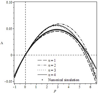
Fig. 2Variation of moment Lyapunov exponent with n and p for the case: k1= 2, k2= 0, k3= 3, k4=1, b13=b23=b31=1, b32=0, b33=1, μ=σ=ω=1, δ1=δ2= 1

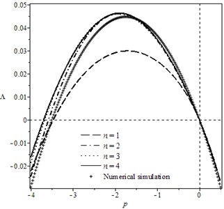
Fig. 3Variation of moment Lyapunov exponent with parameters p and μ for the case: k1= 2, k2= 0, k3= 3, k4=1, b13=b23=b31=1, b32=0, b33=1, σ=ω= 1, δ1=δ2= 1

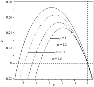
Fig. 4Variation of moment Lyapunov exponent with parameters p and σ for the case: k1= 2, k2= 0, k3= 3, k4=1, b13=b23=b31=1, b32=0, b33=1, σ=ω= 1, δ1=δ2= 1

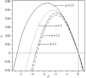
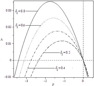
In addition, it can be shown from the expressions of the elements in matrix $A$ that the moment Lyapunov exponents are relevant to the parameters of the system and the noise excitation. Fig. 3 and Fig. 4 describe the effect of noise parameters on the moment Lyapunov exponent. One can easily find that the apexes of the moment Lyapunov exponents move to the left and rise as both $μ$ and $σ$ increase, which illustrates the stability of the system become poor with the increased $μ$ and $σ$ . Moreover, by comparing two figures, we can see the effect of $μ$ is bigger than that of $σ$ . The trend of the curves in Fig. 5 is similar to Fig. 3, but the varied range is less than the one in Fig. 3. Fig.6 displays that the curves of moment Lyapunov exponent transform from the right side of vertical axis to the left with the increase of $δ_{1}$ , and the bigger $δ_{1}$ is, the larger the influence on the moment Lyapunov exponent. Finally, in view of Fig. 7, we see that the peak of the moment Lyapunov exponents moves to the left and ascends rapidly with increase of $δ_{2}$ , and the vary of the curves is also alike to Fig. 3. Therefore, it can be seen from Fig. 3-7 that the parameter $μ$ , $δ_{1}$ and $δ_{2}$ play the significant influence on the moment Lyapunov exponent.

Fig. 5Variation of moment Lyapunov exponent with parameters p and ω for the case: k1= 2, k2= 0, k3= 3, k4= 1, b13=b23=b31= 1, b32= 0, b33= 1, μ=ω= 1, δ1=δ2= 1

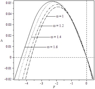
Fig. 6Variation of moment Lyapunov exponent with parameters p and δ1 for the case: k1= 2, k2= 0, k3= 3, k4= 1, b13=b23=b31= 1, b32= 0, b33= 1, μ=σ=ω= 1, δ2= 1

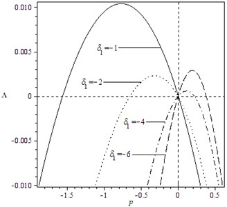
Fig. 7Variation of moment Lyapunov exponent with parameters p and δ2 for the case: k1= 2, k2= 0, k3= 3, k4= 1, b13=b23=b31= 1, b32= 0, b33= 1, μ=σ=ω= 1, δ1= 1

6. Conclusions

In this paper, the moment Lyapunov exponent of a co-dimension two bifurcation system, that is on a three dimensional center manifold and is parametrically excited by a bounded noise, is investigated. By a reversible linear transformation and perturbation method, a corresponding eigenvalue problem and each order perturbation of the moment Lyapunov exponent are obtained. Zero, one and two order perturbation are solved through differential equation and stochastic process theory, thus, the eigenvalue problem of probability density is yielded. Finally, the eigenvalue problem is solved by Fourier cosine series expansion, and an infinite matrix yields and whose leading eigenvalue is the second order perturbation of the moment Lyapunov exponent. Furthermore, the convergence of procedure is numerically verified in two cases. Finally, the effects of system parameters and noise parameters on the expression of the moment Lyapunov exponent are discussed.

References

Molcanov S. A. The structure of eigenfunctions of one-dimensional unordered structures. Mathematics of the USSR – Izvestiya, Vol. 12, 1978, p. 69-101.

Search CrossRef
Arnold L. A formula connecting sample and moment stability of linear stochastic systems. SIAM Journal of Applied Mathematics, Vol. 44, 1984, p. 793-802.

Search CrossRef
Arnold L., Kliemann W., Oejeklaus E. Lyapunov Exponents of Linear Stochastic Systems. Lyapunov Exponents Lecture Notes in Mathematics, Vol. 1186, 1986, p. 85-125.

Search CrossRef
Arnold L., Oejeklaus E. Almost Sure and Moment Stability for Linear Equations. Lyapunov Exponents, Lecture Notes in Mathematics, Vol. 1186, 1986, p. 129-159.

Search CrossRef
Arnold L., Doyle M., Namachchivaya Sri N. Small noise expansion of moment Lyapunov exponents for two-dimensional systems. Dynamics and Stability of Systems, Vol. 12, 1986, p. 187-211.

Search CrossRef
Namachchivaya Sri N., Van Roessel H., Doyle M. Moment Lyapunov exponent for two coupled oscillators driven by real noise. SIAM Journal of Applied Mathematics, Vol. 56, 1996, p. 1400-1423.

Search CrossRef
Khasminskii R., Moshchuk N. Moment Lyapunov exponent and stability index for linear conservative system with small random perturbation. SIAM Journal of Applied Mathematics, Vol. 58, 1988, p. 245-256.

Search CrossRef
Namachchivaya Sri N. Moment Lyapunov exponent and stochastic stability of two coupled oscillators driven by real noise. Journal of Applied Mechanics, Vol. 68, 2001, p. 903-914.

Search CrossRef
Xie W.-C. Moment Lyapunov exponents of a two dimensional system under real noise excitation. Journal of Sound and Vibration, Vol. 239, 2001, p. 139-155.

Search CrossRef
Xie W.-C. Moment Lyapunov exponents of a two dimensional system under bounded noise parametric excitation. Journal of Sound and Vibration, Vol. 263, 2003, p. 593-616.

Search CrossRef
Liu X. B., Liew K. M. On the stability properties of a Van Der Pol-Duffing oscillator that is driven by a real noise. Journal of Sound and Vibration, Vol. 285, 2005, p. 27-49.

Search CrossRef
Higham D., Mao X., Yuan C. Almost sure and moment exponential stability in the numerical simulation of stochastic differential equations. SIAM Journal on Numerical Analysis, Vol. 45, 2007, p. 592-609.

Search CrossRef
Kozic P., Janevski G., Pavlovic R. Moment Lyapunov exponent and stochastic stability of a double-beam system under compressive axial loading. International Journal of Solids and Structures, Vol. 47, 2010, p. 1435-1442.

Search CrossRef
Li S. H., Liu X. B. Moment Lyapunov exponent for a three dimensional stochastic system. IUTAM Symposium on Nonliear Stochastic Dynamics and Control, Vol. 29, 2011, p. 191-200.

Search CrossRef
Li S. H., Liu X. B. Moment Lyapunov exponent for three-dimensional system under real noise excitation. Applied Mathematics and Mechanics, Vol. 34, 2013, p. 613-626.

Search CrossRef
Hu D. L., Huang Y., Liu X. B. Moment Lyapunov exponent and stochastic stability of binary airfoil driven by Non-Gaussian colored noise. Nonliear Dynamics, Vol. 70, 2012, p. 1847-1859.

Search CrossRef
Liew K. M., Liu X. B. The maximal Lyapunov exponent for a three-dimensional stochastic system. Journal of Applied Mechanics, Vol. 71, 2004, p. 677-690.

Search CrossRef
Li S. H., Liu X. B. The maximal Lyapunov exponent for a co-dimensional two-bifurcation system excited by bounded noise excitation. Acta Mechanica Sinica, Vol. 28, 2012, p. 511-519.

Search CrossRef
Guckenheimer G., Holmes P. Nonlinear Oscillations, Dynamical Systems and Bifurcations of Vector Field. Spring-Verlag, New York, 1983

Search CrossRef
Zauderer E. Partial Differential Equations of Applied Mathematics. 2nd Edition, Wiley, New York, 1989.

Search CrossRef
Wedig W. Lyapunov Exponent of Stochastic Systems and Related Bifurcation Problems. Stochastic Structural Dynamics Progress in Theory and Applications. Elsevier Applied Science, New York, 1988, p. 315-327.

Search CrossRef
Bolotin V. V. The Dynamic Stability of Elastic Systems. Holden-Day, San Francisco, 1964.

Search CrossRef
Xie W. C., Huang Q. H. On the Monte Carlo simulation of moment Lyapunov exponents. Advances in Engineering Structures, Mechanics and Construction, Vol. 140, 2006, p. 627-636.

Search CrossRef

About this article

Received

22 April 2015

Accepted

11 August 2015

Published

30 December 2015

SUBJECTS

Chaos, nonlinear dynamics and applications

Keywords

moment stability

moment Lyapunov exponent

perturbation method

diffusion process

This is an open access article distributed under the Creative Commons Attribution License, which permits unrestricted use, distribution, and reproduction in any medium, provided the original work is properly cited.