Vibration control for active magnetic bearing high-speed flywheel rotor system with modal separation and velocity estimation strategy

1. Introduction

In the flywheel energy storage system, a high-speed flywheel is widely used to store energy. The flywheel energy storage systems are suitable whenever numerous charge/discharge cycles (hundreds of thousands) are needed with medium to high power (kW to MW) during the short period (tens of seconds).

In order to maximize the energy density and storage efficiency, the rotating speed of the flywheel rotor should be as high as possible and the polar moment of inertia of the flywheel rotor should be as large as possible. Active magnetic bearing (AMB) is the best choice for the supporting structure of a high-speed flywheel energy storage system due to its no contact, no wear, no need of lubrication and dynamic adjustable. Therefore, the high-speed flywheel which is supported on active magnetic bearings and made by composite materials is considered as a promising and attracting one.

In the AMB high-speed flywheel rotor system, there is a strong coupling between conical mode and parallel mode, which would weaken the stability and control performances of the AMB high-speed flywheel rotor system. Besides, the gyroscopic effect becomes more significant because of the high ratio of polar to transverse moments of inertia of the flywheel rotor and high rotating speed. However, the strong gyroscopic effect greatly increases the complexity of the control system, and may result in rotor instability in some cases [1]. Traditional decentralized controllers, such as proportional-derivative controller (PD controller), are very difficult to deal with such complex system due to the strong coupling between different rigid modes and the gyroscopic effect [2-4]. In order to improve the stability and control performances, it is necessary to develop some advanced control methods.

Various control methods have been studied in the past few decades. They are classified into two kinds, one is based on the modern control theory and intelligent control theory, such as sliding mode control [5, 6], $\mu$ synthesis control [7, 8], robust gain-scheduled $H_{\infty }$ control [9, 10], LQR control [11], adaptive control [12], optimal control [13,14], feedback linearization control [15], fuzzy logic control [16, 17]. These control methods can get a good control performance, but they are difficult to realize due to the complexity of control algorithm. The other is based on the traditional decentralized control, such as cross-feedback control [18-20], two-degree-of-freedom PID control [21, 22], which has a simple structure, but designing a good controller is not so easy due to the strong coupling between conical mode and parallel mode of the AMB high-speed flywheel rotor system.

In order to eliminate the coupling between conical mode and parallel mode of the AMB high-speed flywheel rotor system, modal decoupling control was presented [23, 24], however, this control strategy has poor robustness against noise. In this paper, a new control strategy based on modal separation and velocity estimation was proposed for the AMB high-speed flywheel rotor system. Firstly, the mathematical model of a four-degree-of-freedom vertical AMB high-speed flywheel rotor system was developed, then, the principle and realization of the proposed control strategy was introduced based on this model. The modal separation is used to cancel the coupling between conical mode and parallel mode of the AMB flywheel rotor system, and the velocity estimation controller is adopted to achieve high robustness against noise. Finally, comparative simulations and experiments have been developed to evaluate the effectiveness and superiority of the proposed control strategy.

2. Model of the AMB high-speed flywheel rotor system

In most AMB high-speed flywheel energy storage systems, the bending critical speed of flywheel rotor system is much higher than the operating speed, so the flywheel rotor system is often considered as a rigid rotor. The simplified model of a vertical AMB flywheel rotor system is shown in Fig. 1. The flywheel rotor system is supported axially by a pair of permanent magnetic (PM) bearings located on the top and bottom sides, and radially by two AMBs.

Fig. 1Schematic of the AMB high-speed flywheel rotor system

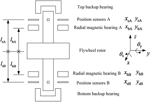
In order to describe the motions of the AMB flywheel rotor system, it is assumed that the axial line of the flywheel rotor is centralized as the geometric center line of the two radial AMBs. Three coordinate systems are defined, which are sensor coordinate systems $o_{sA}{x}_{sA}{y}_{sA}$ and $o_{sB}{x}_{sB}{y}_{sB}$, radial AMB coordinate systems $o_{bA}{x}_{bA}{y}_{bA}$ and $o_{bB}{x}_{bB}{y}_{bB}$, and mass center coordinate system $oxyz$, respectively. All original points of the three coordinate systems are in the geometric center line of the two radial AMBs. The original point of mass center coordinate system $oxyz$ is fixed to the mass center of the flywheel rotor system and $z$ axis to the spinning axis of the flywheel rotor system. The $x$ and $y$ denote translation displacements of mass center of the flywheel rotor along $x$ and $y$ axes, respectively, while ${\theta }_x$ and ${\theta }_y$ are angular displacements of the flywheel rotor about $x$ and $y$ axes. In the sensor coordinate systems, the displacements of the flywheel rotor at the upper and the lower sensor positions are ($x_{sA}$, $y_{sA}$) and ($x_{sB}$, $y_{sB}$), respectively. Similarly, in the radial AMB coordinate systems, the displacements of the flywheel rotor at the upper and the lower radial AMB positions are ($x_{bA}$, $y_{bA}$) and ($x_{bB}$, $y_{bB}$). The relative positions between the sensors, the radial AMBs and the mass center of the flywheel rotor system are also shown in Fig. 1. $l_{bA}$ is the distance between the central point $o_{bA}$ of the magnetic bearing A and the mass center $o$, while $l_{bB}$ is the distance between the central point $o_{bB}$ of the magnetic bearing B and the mass center $o$. Similarly, $l_{sA}$ refers to the distance between the central point $o_{sA}$ of the position sensors A and the mass center $o$, and $l_{sB}$ is the distance between the central point $o_{sB}$ of the position sensors B and the mass center $o$.

In order to simplify theoretical analysis, the following assumptions are made: a) the flywheel rotor system is a rigid rotor; b) the coupling between the axial PM bearings and radial AMBs is neglected; c) the radial AMBs are symmetrical in geometry for $x$ and $y$ axes, and there is no coupling between magnetic poles in the radial AMBs; d) the radial AMBs magnetic forces are simplified as a linear model.

For the motions of the AMB high-speed flywheel rotor in radial directions, the equation of motion is:

where $m$ is the total mass of the flywheel rotor, $J_x$ and $J_y$ are transverse moments of inertia of the flywheel rotor around $x$ and $y$ axes, respectively, $J_z$ is the polar moment of inertia of the flywheel rotor around $z$ axis, $w$is the rotating speed about spinning axis $z$. $f_{xA}$, $f_{yA}$, $f_{xB}$ and $f_{yB}$ are magnetic forces acting on the flywheel rotor in the upper and lower radial AMB positons.

The matrix form of the equation of motion of the AMB flywheel rotor system is:

where:

Generally, the magnetic forces produced by radial AMBs ($f_{xA}$, $f_{yA}$, $f_{xB}$ and $f_{yB}$) can be simplified as a linear model, which is:

where $k_{sA}$ and $k_{iA}$ are the force-displacement coefficient and the force-current coefficient of the upper radial AMB, respectively, while $k_{sB}$, and $k_{iB}$ are the force-displacement coefficient and the force-current coefficient of the lower radial AMB.

The matrix form of Eq. (3) is:

where:

are force-displacement matrix and force-current matrix of the AMBs, respectively. $\mathbf{I}={\left[i_{xA}{i}_{xB}{i}_{yA}{i}_{yB}\right]}^T$ is the control current vector. ${\mathbf{q}}_b={\left[x_{bA}{x}_{bB}{y}_{bA}{y}_{bB}\right]}^T$ is the displacement vector of the flywheel rotor at the upper and the lower radial AMB positions in the radial AMB coordinate systems, the coordinate transformations between the radial AMB coordinates ($x_{bA}$, $x_{bB}$, $y_{bA}$ and $y_{bB}$) and the mass center coordinates (${\theta }_y$, $x$, ${\theta }_x$ and $y$) is:

The combination of Eq. (2) with Eq. (4) and Eq. (5) yields:

where:

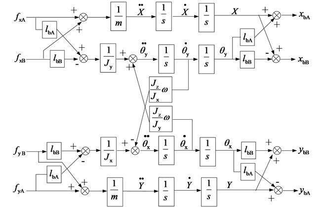
The function block diagram based on the equation of motion of the AMB high-speed flywheel rotor system is shown in Fig. 2. It is shown that the conical mode (${\theta }_y$, ${\theta }_x$) and the parallel mode ($x$, $y$) of the AMB flywheel rotor system are coupled to each other. Since the conical mode and the parallel mode have different characteristics and control objectives. In order to get better control performances, the control strategy of modal separation is needed.

For the decentralized PD control, output control current is:

where ${\mathbf{q}}_s={\left[x_{sA}{x}_{sB}{y}_{sA}{y}_{sB}\right]}^T$ is the displacement vector of the flywheel rotor at the upper and the lower sensor positions in sensor coordinate systems. $\mathbf{P}=\mathrm{d}\mathrm{i}\mathrm{a}\mathrm{g}\left(p_{xA}{p}_{xB}{p}_{yA}{p}_{yB}\right)$ is the proportional gain coefficient matrix, $\mathbf{D}=\mathrm{d}\mathrm{i}\mathrm{a}\mathrm{g}\left(d_{xA}{d}_{xB}{d}_{yA}{d}_{yB}\right)$ is the differential gain coefficient matrix. Generally, the radial AMBs are symmetrical in geometry for $x$ and $y$ axes, i.e., $p_{xA}=p_{yA}=p_A$, $p_{xB}=p_{yB}=p_B$, $d_{xA}=d_{yA}=d_A$, $d_{xB}=d_{yB}=d_B$, thus the proportional gain coefficient matrix $\mathbf{P}$ and differential gain coefficient matrix $\mathbf{D}$ can be simplified as $\mathit{P}=\mathrm{d}\mathrm{i}\mathrm{a}\mathrm{g}\left(p_A{p}_B{p}_A{p}_B\right)$ and $\mathbf{D}=\mathrm{d}\mathrm{i}\mathrm{a}\mathrm{g}\left(d_A{d}_B{d}_A{d}_B\right)$.

Fig. 2Function block diagram of the AMB flywheel rotor system

Substituting Eq. (7) into Eq. (6) yields:

The coordinate transformations between the sensor coordinates ($x_{sA}$, $x_{sB}$, $y_{sA}$ and $y_{sB}$) and the mass center coordinates of the AMB flywheel rotor system (${\theta }_y$, $x$, ${\theta }_x$ and $y$) is given by:

where:

Submitting Eq. (9) to Eq. (8), one obtained:

The Eq. (10) can be rewritten as:

In order to simplify the expression of Eq. (11), we introduce two substitution matrices ${\mathbf{K}}_C$ and ${\mathbf{D}}_C$, and let ${\mathbf{K}}_c={\mathbf{L}}_f{\mathbf{K}}_i\mathbf{P}{\mathbf{T}}_s$, ${\mathbf{D}}_c={\mathbf{L}}_f{\mathbf{K}}_i\mathbf{D}{\mathbf{T}}_s$, then Eq. (11) can be simplified as:

where:

It is clear that ${\mathbf{K}}_c$ and ${\mathbf{D}}_c$ can be considered as the stiffness and the damping matrices provided by the PD controller. The stiffness matrix should be large enough to compensate the negative bearing stiffness matrix –${\mathbf{K}}_{ss}$ in order to yield closed-loop eigenvalues located on the imaginary axis. The damping matrix ${\mathbf{D}}_c$ should be positive in order to make the system be asymptotically stable, i.e. to achieve closed-loop eigenvalues entirely located in the left half of the complex plane. From the expressions of ${\mathbf{K}}_c$ and ${\mathbf{D}}_c$, we can learn that the conical mode and parallel mode are coupled together, so the decentralized PD controller could not direct control over the rotor rigid modes.

3. Proposed control strategy

3.2. Velocity estimation controller

In section 3.1, the PD controller uses the derivative of position signal of the flywheel rotor to generate its damping control signal. However, the noisy nature of derivative results in a noise plagued damping signal. This impacts flywheel controllability, as the levitated flywheel cannot be damped adequately without introducing noise. Therefore, the velocity estimator controller is developed specifically to improve the quality of the damping control effort, mainly to reduce the noise in the damping signal. The implementation of PD controller and velocity estimation controller are shown schematically in Fig. 3, respectively.

Fig. 3Implementation of PD controller and velocity estimation controller

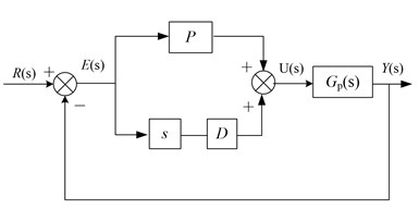
a) PD controller

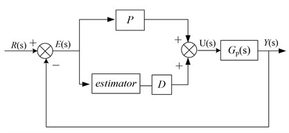
b) Velocity estimation controller

In Fig. 3, $G_p\left(s\right)$ represents the control object, and the “estimator” term is the velocity value of flywheel rotor calculated by the velocity estimator. Note that there is a similarity between the velocity estimation controller and the PD controller; for the velocity estimation controller, the derivative is simply replaced by the estimator value. The algorithm of the velocity estimator can be formulated as:

27

$\left\{\begin{array}{l}{\dot{x}}_1\left(t\right)=x_2\left(t\right),\\ {\dot{x}}_2\left(t\right)=R^2\left[-{\alpha }_0\left(x_1\left(t\right)-e\left(t\right)\right)-{\alpha }_1{x}_1\left(t\right)-e\left(t\right){)}^{\frac{n}{m}}-{\alpha }_2{\left(\frac{x_2\left(t\right)}{R}\right)}^{\frac{n}{m}}\right],\end{array}\right.$

where $e\left(t\right)$ is the position signal, $x_1\left(t\right)$ and $x_2\left(t\right)$ represent the estimated states, that is, $x_1\left(t\right)=e\left(t\right)$, $x_2\left(t\right)=\dot{e}\left(t\right)$. $R$, ${\alpha }_0$, ${\alpha }_1$, ${\alpha }_2$, $m$ and $n$ are constant coefficients, which $R>$ 0, ${\alpha }_0$, ${\alpha }_1$, ${\alpha }_2>$ 0, and $m>n$ are positive odd numbers. Convergence speed can be improved by increasing the coefficients $R$, ${\alpha }_0$, ${\alpha }_1$, ${\alpha }_2$,however, the noise would be introduced as the increasing of the coefficients $R$, ${\alpha }_0$, ${\alpha }_1$, ${\alpha }_2$.

The schematic diagram of the algorithm of the velocity estimator is shown in Fig. 4.

Fig. 4Velocity estimator schematic

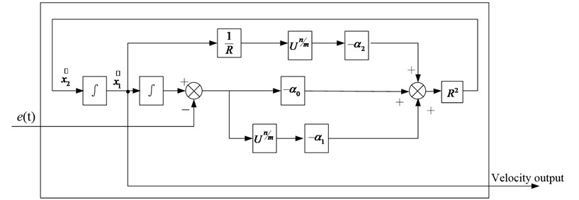
As can be seen in Fig. 4, the velocity output (damping control signal) is obtained by numerical integration, and numerical integration can provide more stable and accurate results than numerical differentiation in the presence of noise. So, the velocity estimator controller can reduce the noise in the damping signal.

3.3. Realization of the proposed control strategy

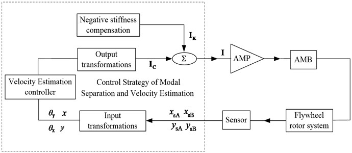
A simplified schematic of the proposed control strategy is shown in Fig. 5. In Fig. 5, AMP stands for power amplifier, while AMB represents active magnetic bearing. The proposed control strategy mainly includes four function modules: the module of negative stiffness compensation, input transformation module, velocity estimation controller and output transformation module. The displacements of the flywheel rotor system are measured by eddy current sensors, and these sensor signals are fed back to the controller. Firstly, the module of negative stiffness compensation produces the compensation current ${\mathbf{I}}_k$ to cancel the effect of the negative stiffness of AMBs. Then, an input transformation is performed at the input side of the controller to convert the sensor displacements to mass center displacements of the flywheel rotor system. Subsequently, the velocity estimation controller processes the mass center displacement signals of the flywheel rotor system and generates the modal control current. Finally, an output transformation is employed at the output side of the controller to convert the modal control current about mass center coordinate system to the current ${\mathbf{I}}_c$ about AMB coordinate system. The sum of modal control current ${\mathbf{I}}_c$ and compensation current ${\mathbf{I}}_k$ is the total control current $\mathbf{I}$, and the total currents $\mathbf{I}$ is converted to drive current by the AMP. The drive current is fed to the AMB, forces produced by the AMB suspend the flywheel rotor system.

Fig. 5Schematic diagram of the proposed control strategy

4. Simulation and experiment results

Comparative simulations and experiments among the decentralized PD controller and the proposed control strategy have been carried out in this section to evaluate the performances of the proposed control strategy.

4.1. Experimental setup

Extensive experiments have been performed on an AMB high-speed flywheel energy storage system shown in Fig. 6.

Fig. 6AMB high-speed flywheel energy storage system and its flywheel rotor

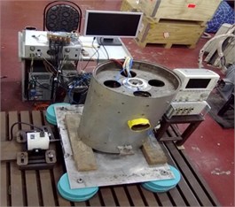
a) AMB high-speed flywheel energy storage system

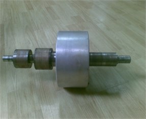
b) Flywheel rotor

The AMB flywheel rotor system of this flywheel energy storage system includes a flywheel rotor, two radial AMBs, four eddy-current sensors, a bearing controller and a switching power amplifier.

The flywheel rotor system is supported axially by a pair of PM bearings located on the top and the bottom sides, and radially by two AMBs.

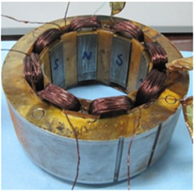
The two radial AMBs have the same geometry, and the structure of radial AMB is the conventional eight pole arrangements, as shown in Fig. 7. The differential excitation currents are employed to drive the AMBs. In this case, the force-displacement coefficient and the force-current coefficient can be calculated as follows:

28

$\left\{\begin{array}{l}{k}_{sA}=k_{sB}=\frac{{\mu }_{0}A{N}^2{I}_0^2\mathrm{c}\mathrm{o}{\mathrm{s}}^2\alpha }{C_0^3},\\ k_{iA}=k_{iB}=\frac{{\mu }_{0}A{N}^2{I}_0\mathrm{c}\mathrm{o}\mathrm{s}\alpha }{C_0^2},\end{array}\right.$

where ${\mu }_0$ is the permeability of vacuum, $A$ is the pole area, $N$ is the coil turns of a pair of pole, $I_0$ is the bias current, $\alpha$is the angle of each pole relative to the centerline between the poles, and $C_0$ is the nominal air gap length. In this setup, the parameters are as follows: $C_0=$0.3×10^-3m, $A=$ 0.225×10^-3 m², $N=$ 100, $I_0=$1.3 A, $\alpha =$ 22.5°.

Fig. 7The structure of radial active magnetic bearing

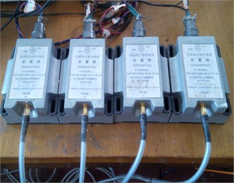
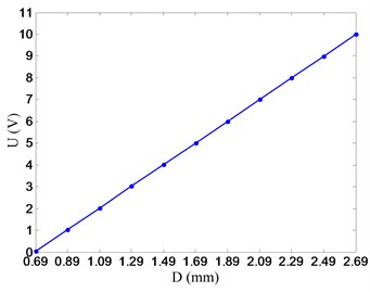
The rotor positions are measured by four eddy-current displacement sensors, i.e., two sensors are mounted near the upper radial magnetic bearing, and the other two sensors are placed near the lower radial magnetic bearing. The two sensors located in the same side (upper side or lower side) are mounted in mutually perpendicular directions to measure the displacements of the flywheel rotor along $x$ and $y$ axes, respectively. Fig. 8 shows the four eddy-current displacement sensors and the input-output characteristic curve.

The input-output characteristic curve of the eddy-current displacement sensor is shown in Fig. 8(b). $D$ represents the displacement between the sensor probe and the flywheel rotor. $U$, the output of the eddy-current displacement sensor, is a voltage signal. The relationship between input signal $D$ and output signal $U$ is:

29

$U=4.975\times D-3.397.$

In Eq. (29), the units of input $D$ and output $U$ are millimeter and volt, respectively.

DS1103 PPC is adopted as the bearing controller to generate command signals. It is provided by the dSPACE company in Germany. The DS1103 PPC has the advantages of strong real-time, high reliability and easy to expansion. It has 20 analog-to-digital converters (ADC) and 8 digital-to-analog converters (DAC). The sampling times of the ADC and DAC are 4 s and 5 s, respectively. The input voltage of the ADC is ±10 V, and the output voltage of the DAC is also ±10 V.

Fig. 8Eddy current sensors and input-output characteristic curve

a) The eddy-current displacement sensors

b) Input-output characteristic curve of the eddy-current displacement sensor

The basic parameters of the AMB high-speed flywheel energy storage system are as follows: rated power $P_N=$10 kw, rated speed $n_N=$20000 rpm, efficiency $\eta =$95 %, rated voltage $U_N=$400 V. The parameters of the AMB flywheel rotor system are shown in Table 1. In Table 1, $k_{iA}$, $k_{iB}$, $k_{sA}$ and $k_{sB}$ are calculated by Eq. (28).

Table 1Basic parameters of the AMB flywheel rotor system

Parameter	Symbol	Value	Unit
Total mass	$m$	25.8	kg
Transverse moment of inertia	$J_x=J_y$	0.2388	kg m2
Polar moment of inertia	$J_z$	0.1151	kg m2
Distance between the central point of AMB and mass center o	$l_{bA}=l_{bB}$	200	mm
Distance between the central point of sensors and mass center o	$l_{sA}=l_{sB}$	240	mm
Force-current coefficient	$k_{iA}=k_{iB}$	37.7	NA-1
Force-displacement coefficient	$k_{sA}=k_{sB}$	15.08×104	Nm-1

4.2. Simulation results

4.2.1. Modes analysis

The AMB flywheel rotor system in both no-rotating and rotating cases has two kinds of natural rigid modes, i.e., the conical mode and the parallel mode. The conical mode describes rotor tilt around its mass center. The parallel mode describes the translation motions of the rotor mass center in $x$, $y$ plane, no tilting around its mass center. When the rotor is spinning, the parallel mode frequency does not change much with the rotating speed, but the conical mode separates into nutation mode and precession mode with the increase of rotating speed. The nutation mode rotates in the same direction as rotor rotation, while the precession mode in the opposite direction as rotor rotation. The nutation mode frequency increases with the rotating speed, while the precession mode frequency decreases with rotating speed [1]. The variation of eigenvalues of the AMB flywheel rotor system with the rotating speed is shown in Fig. 9, where $\sigma$and $j\omega$are real part and imaginary part of the eigenvalue, respectively. The real part of the eigenvalue stands for the stability of the AMB flywheel rotor system and the imaginary part for the vibration frequency. The stiffness of the AMB flywheel rotor system mainly influences the vibration frequency, i.e. the imaginary part of the eigenvalue $j\omega$. The damping of the AMB flywheel rotor system, on the other hand, moves both eigenvalues into the left half of the complex plane, i.e. influence the real part of the eigenvalue $\sigma$. In Fig. 9, the two circles standing for the conical mode and two stars standing for the parallel mode are the eigenvalues of the AMB flywheel rotor system without rotating. The real parts and imaginary parts of eigenvalues of the nutation mode in solid line increase with the rotating speed, while the real parts and imaginary parts of eigenvalues of the precession mode in dashed line decrease with rotating speed. The real parts and imaginary parts of eigenvalues of the parallel mode do not change with the increase of rotating speed.

In the high rotating speed region, the nutation mode with a high frequency is very difficult to control and may result in system instability due to phase lag in the control system and limited bandwidths of the power amplifiers and sensors. Besides, both the real parts and imaginary parts of the precession mode approach to zero, the stability of the AMB flywheel rotor system becomes very weak, and may also result in rotor instability due to the small damping. Finally, there is even a third undesired property, as seen in Fig. 9, the damping over the two rigid modes is very unequal distribution, i.e. the conical mode features a very adequate real parts of their eigenvalues already at standstill, whereas the parallel mode remains only very weakly damped. The small damping of the parallel mode may also result in rotor instability in the control system. So, it is necessary to regulate the rigid modes’ stiffness (frequency) and damping independently.

Fig. 9Variation of eigenvalues of the AMB flywheel rotor system with rotating speed

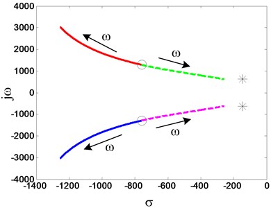
Fig. 10Variation of mode frequency with P for decentralized PD control at 20000 rpm

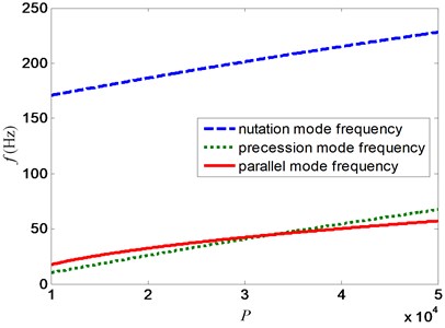
Fig. 11Variation of mode frequency with pcon for proposed control strategy at 20000 rpm

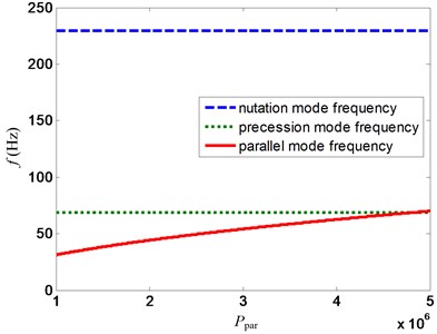
Fig. 12Variation of mode frequency with ppar for proposed control strategy at 20000 rpm

Because the methods of regulating the rigid modes’ stiffness and damping are similar to each other, in this paper, the regulating process of the rigid modes’ stiffness was taken as an example. The variation of mode frequencies of the AMB flywheel rotor system for the decentralized PD control with the proportional coefficient $P$ at 20000 rpm is shown in Fig. 10. As seen in the figure, both the conical mode frequencies, i.e. the nutation mode frequency and the precession mode frequency, and the parallel mode frequency increase when the proportional coefficient $P$ rises up. Therefore, the decentralized PD control could not separately regulate the rigid modes’ frequencies of the AMB flywheel rotor system.

The variations of mode frequencies of the AMB flywheel rotor system with the proportional coefficient $p_{con}$ and $p_{par}$ for the proposed control strategy are shown in Fig. 11 and 12, respectively. It is demonstrated that the conical mode frequencies, i.e., the nutation mode frequency and the precession mode frequency, increase as the increase of $p_{con}$, whereas the parallel mode frequency always remains a constant. And vice versa, the parallel mode frequency also increases as the increase of $p_{par}$, while the conical mode frequencies still remain a constant. Hence, the conical mode control channel and the parallel mode control channel are totally independent, which allow us to regulate the different rigid modes’ frequencies through changing the proportional coefficient of the corresponding mode control channel.

4.2.2. Dynamic characteristics and stability

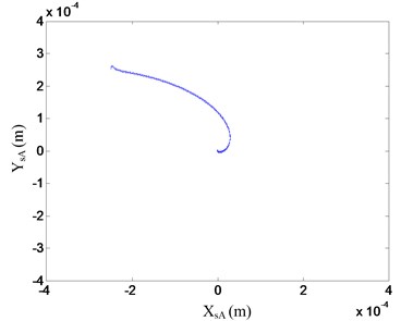
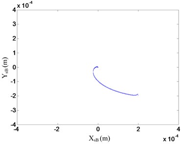
In order to investigate the dynamic characteristics and stability, the decentralized PD controller and the proposed control strategy were employed to control the flywheel rotor system, respectively. In this simulation, the initial positions of the flywheel rotor system in the sensor coordinates are [$x_{sA}{x}_{sB}{y}_{sA}{y}_{sB}$] $=$ [–0.25 0.2 0.25 –0.2] mm. The orbits and vibrations of the flywheel rotor system with a suitable decentralized PD controller at 20000 rpm are shown in Fig. 13 and 14, respectively.

Fig. 13Orbit of the flywheel rotor with decentralized PD controller at 20000 rpm

a) Orbit of A plane

b) Orbit of B plane

Fig. 14Vibrations of the flywheel rotor with decentralized PD controller at 20000 rpm

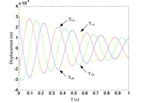
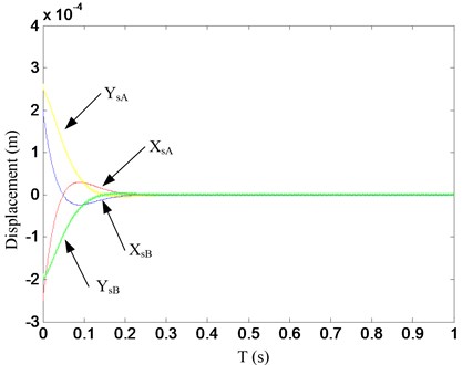
The orbits and vibrations of the flywheel rotor system with proposed control strategy are shown in Fig. 15 and 16. As seen in these figures, for the decentralized PD controller, the flywheel rotor system tends to loose stability, the overshoots and vibrations of the flywheel rotor system are large at this rotational speed. However, the stability, overshoot and vibrations of the flywheel rotor system can be greatly improved with the proposed control strategy. It also takes a short time for flywheel rotor to reach the reference positions, i.e., the adjusting time is short with the proposed control strategy. So, the proposed control strategy has better stability and dynamic characteristics.

Fig. 15Orbit of the flywheel rotor with proposed control strategy at 20000 rpm

a) Orbit of A plane

b) Orbit of B plane

Fig. 16Vibrations of the flywheel rotor with proposed control strategy at 20000 rpm

4.2.3. Robustness against noise

The main difference between the PD controller and velocity estimation controller is how to get the velocity signal. The PD controller uses the derivative of position signal of the flywheel rotor to generate its velocity signal; while the velocity estimation controller obtains it by means of velocity estimator. Therefore, the difference of robustness against noise of the two controllers mainly depends on differentiator and velocity estimator. To evaluate the robust against noise of the proposed control strategy, a sinusoidal signal with white noise was fed to the differentiator and velocity estimator, respectively, and the outputs (velocity signals) of differentiator and velocity estimator were stored. The frequency of sinusoidal signal is 50 Hz, this is well within the bandwidth of the AMB, and so the AMB flywheel rotor system may operate at this speed. The amplitudes of sinusoidal signal and white noise are 1 and 0.05, respectively. Fig. 17 shows the outputs of differentiator and velocity estimator with white noise sine wave as the input. Since the output is the velocity of the input signal, ideally the outputs of differentiator and velocity estimator should be sinusoidal. In Fig. 17, output of velocity estimator is clearly sinusoidal in shape. However, with the differentiator response, the sine wave is almost undetectable due to the effect of white noise; there is considerably more noise in the output of differentiator. Because the outputs of differentiator and velocity estimator are damping control signals provided by PD controller and velocity estimation controller, respectively. So, compared with PD controller, the estimation controller has stronger robustness against noise.

Fig. 17Outputs of differentiator and velocity estimator with white noise sine wave as the input

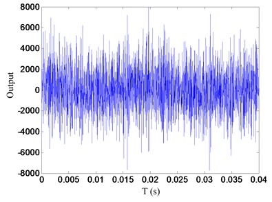
a) Output of differentiator

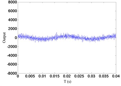
b) Output of velocity estimator

4.3. Experimental results

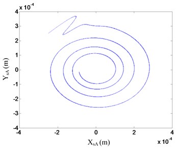
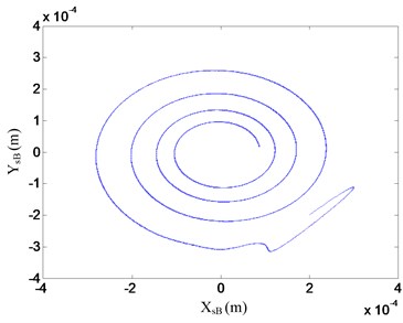
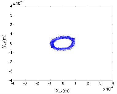
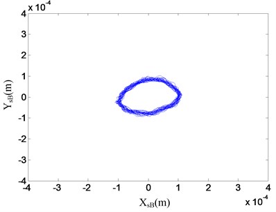
In order to validate the control performances of the proposed control strategy, the decentralized PD control and the proposed control strategy were used for the operation of the AMB high-speed flywheel energy storage system, respectively. In the process of experiment, ten thousand displacement data were stored per second for each displacement sensor by means of DS1103 PPC. Then with the displacements in $x$ direction ($x_{sA}$ or $x_{sB}$) as $x$-axis and the displacements in $y$ direction ($y_{sA}$ or $y_{sB}$) as $y$-axis, we can plot the orbits of the flywheel rotor system by MATLAB. Orbits of the AMB flywheel rotor system with the decentralized PD control at 20000 rpm are shown in Fig. 18. The orbits of AMB flywheel rotor system with the proposed control strategy at the same speed are shown in Fig. 19. As can be seen from the two figures, at this rotational speed, the vibrations of the flywheel rotor system with the proposed control strategy are much smaller than that of the flywheel rotor system with the decentralized PD controller, and there are considerably less noises in the position signals of flywheel rotor system with the proposed control strategy.

Fig. 18Orbit of the flywheel rotor with the decentralized PD controller at 20000 rpm in experiments

a) Orbit of A plane

b) Orbit of B plane

Fig. 19Orbit of the flywheel rotor with the proposed control strategy at 20000 rpm in experiments

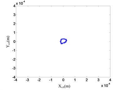
a) Orbit of A plane

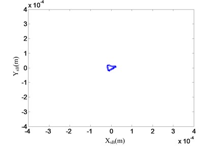
b) Orbit of B plane

5. Conclusions

A new control strategy based on modal separation and velocity estimation was presented in this paper. The principle and realization of the proposed control strategy was introduced based on the mathematical model of the AMB high-speed flywheel rotor system. Comparative simulation and experiment results show that, compared with the traditional method, the proposed control strategy has the following characteristics.

1) It can realize the decoupling between the conical mode and parallel mode of the AMB high speed flywheel rotor system, and can realize separate control of the stiffness and damping of the rotor rigid modes.

2) It has better stability, dynamic characteristics and stronger robustness against noise.

3) It has a simple structure and is easy to implement.

In a word, the proposed control strategy can effectively realize excellent stability, dynamic behaviors and strong-robustness of the AMB high-speed flywheel rotor system without high control effort.