Abstract
There is no doubt that remaining useful life prediction is important to the health management of modern mechanical equipment. But in most cases, the useful operational information of equipment we can get are limited, one of them is vibration signal. Particle filter is a hybrid prediction method combined with data-driven and model-based two kinds of methods. It can solve prognosis problem with the fitted prediction model only by historical data, and allow the uncertainty management. However, the prediction performance of the method is largely dependent on the prediction model and very sensitive to the initial distribution of the model parameters. These flaws limit the further development of particle filter methods in the prediction. Aiming at the shortcomings of the basic particle filter prediction method, a general prediction framework of particle filter based on degradation rate tracking is proposed in this paper. It turned away from the fitted model, and utilized the statistical rule of degradation rate of historical data to estimate and predict the degradation process of system. The effectiveness of the method proposed is validated with useful life prediction case of rolling bearings.
1. Introduction
The structures of modern engineering systems become more complex, and it is difficult to guarantee their long-term operation safety. The failure of a little component may result in the accident of the whole system as well as huge losses and hazards. To avoid accidents, it is necessary to predict the remaining useful life (RUL) of equipment and develop corresponding maintenance schemes of improving the reliability and security of the system and reducing the maintenance cost. Thus, in many important areas, prognosis for faults and the remaining useful life of equipment has been increasingly concerned [1].
In recent years, a lot of methods based on different theories have been developed for the prediction of remaining useful life of machinery [2], including neural networks [3], ARMA time series model [4], half hidden Markov model [5], Relevance Vector Machine [6], and other data-driven approaches as well as physical model-based approaches which are directly used to predict RUL through analytical modeling or simulation of specific components [7-9].
Particle filter (PF) is a kind of nonlinear filtering based on sequential Monte Carlo method. It gets rid of the limitation that the random variables must satisfy the Gaussian distribution while solving nonlinear filtering problems. Hence PF can express much more distributions than the Gaussian model and has stronger modeling capabilities for nonlinear characteristic of the variables. It has been successfully applied to target tracking, aerospace, robotics positioning, fault detection, and other fields and has been also applied to predict faults and useful life for mechanical or electrical instruments recently [9-11]. In 2007, Orchard et al used PF to predict the crack propanation in turbine engine blade and in a UH-60 planetary gear carrier plate with deterministic crack growth model based on Paris’s Law [9]. Saha et al used the relevance vector machine (RVM) and a PF to predict RUL of lithium-ion batteries. In their method, PF isused to estimate the RUL with a state-space model based on impedance spectroscopy data [12]. Then He and Chen et al. utilized PF to predict RUL of lithium-ion batteries with a new model consisting of two exponential functions [13, 14].
Nevertheless, PF is still not mature enough. The problems of PF include the choice of importance function, the degeneracy problem and other problems of the algorithm itself [9]. Moreover, in its application of long-term prediction, the prediction efficacy relies on prediction model excessively and is much sensitive to the initial distribution of the model parameters [13, 15]. The applications of PF in the useful life prediction for machinery are largely limited because condition monitoring for mechanical equipment mainly involves vibration signals and are seriously influenced by external noise. Moreover, in the application, its modeling is difficult and clear degradation characteristics are not available. In this paper, we presented a general prediction framework of degradation rate tracking-based particle filter (DRT-PF) to solve above problems and applied the method in the RUL prediction of mechanical components.
The paper is organized as follows. In Section 2, the characteristics and the implementation of the prediction method based on PF are introduced briefly. In Section 3, the shortcomings of the basic PF prediction method and corresponding improved methods are analyzed. In Section 4, three instances of the PHM 2012 Data Challenge are investigated to validate the developed method for estimating the remaining useful life of rolling bearings, and the investigation results are analyzed. Finally, conclusions are drawn in Section 5.
2. Short overview of particle filter
Since the bootstrap particle filter was proposed by Gordon et al. in the 1990s [16], the PF algorithm has already attracted wide attention. PF became a research focus and a number of improved algorithms were developed. Subsequently, PF was applied in prediction. Based on the Bayesian filtering and Monte Carlo algorithm, the predicted value of the posterior probability density was obtained by time updating and measurement updating.
2.1. Optimal Bayesian filtering
Supposing that the dynamic system can be described by a mathematical model, the state equation and measurement equation are expressed as follows:
where : is the nonlinear function of the system state ; is stationary noise; and are the dimensions of the state and process noise, : is the nonlinear function of the system state ; is stationary noise; and are respectively the measurement dimension and observation noise dimension.
If the initial PDF of the state is known as , then the state prediction equation is:
The state updating equation is:
where:
2.2. Sampling
With Monte Carlo method, the integral calculation can be converted into a summation operation of limited samples. If is the first-order Markov process with easy sampling, its probability density distribution is known and the same to . Supposing that we can extract samples from the probability density distribution , then the posterior probability density distribution of the state is obtained approximately by Eq. (5):
where is the weight of (; is the Dirac function; is the weight of normalized samples:
If , then just depends on and :
In the standard filtering algorithm, take:
Then, the weight , normalized weight , and posterior probability density can be respectively expressed as follows:
2.3. Resampling
One of the main difficulties in the development of PF is the degeneracy problem. As the algorithm evolves in time, the weight variances increase and the importance weight may be concentrated on a small number of particles. Therefore, the predicted value becomes progressively more skewed from the real value. In order to solve the degeneracy problem and adapt the dynamic process of the system, a resampling algorithm is performed to eliminate particles with small weights and duplicate those with large ones. The number of effective particles is defined as:
Whenever , a resampling algorithm is performed. Smaller means more serious degeneracy. is a fixed threshold and is generally set to be . is the number of particles. The stratified resampling algorithm proposed by Carpenter et al. can improve the accuracy of PF algorithm and cut down computational time [17]. If considering residual information, the stratified resampling algorithm will be more reasonable. Therefore, in this paper, stratified resampling algorithm considering residual information is used for PF.
2.4. The implementation steps of the prediction algorithm based on particle filter
In the prediction strategy of system state with PF, the prediction model is determined firstly, and then model parameters are filtered based on known observations. Through iterative updating, model parameters are approximated to the real value as possible. Finally, the estimated values of model parameters are substituted into the prediction model to extrapolate and predict the trend of system degradation state. The steps are described as follows:
Step 1. Extracting degradation features. According to the raw measurement data, the proper degradation features are chosen and extracted for predictive modeling.
Step 2. Obtaining the priori model knowledge. With the extracted degradation features, based on historical data or experiences, the prediction model as well as the initial distribution of the model parameters is determined.
Step 3. Initialization of particle samples. The particle population is randomly generated with the priori probability , and the weight of every particle is .
Step 4. Recursive prediction. The state at time is predicted with the state equation.
Step 5. Updating the particles’ state. Given the current observation, the likelihood function of particles and the observation value are calculated. Accordingly, the particle weights are updated and normalized to obtain the least square estimate of state at time as .
Step 6. Resampling. Resampling is performed according to the particle weights to obtain a new set of particles.
Step 7. At the time , if there is a new observation, go back to Step 2, otherwise go to Step 8.
Step 8. The statistical results of the prediction. All particles are extrapolated for prediction with the prediction model and estimations of model parameters until the specified time or a preset threshold is reached. The statistics of the predicted value or the time when the specified threshold of particles is reached were performed to obtain PDF of at specified time or the PDF of time to exceed a threshold.
3. DRT-PF framework for RUL prediction
3.1. Shortcomings of the basic particle filter prediction method
Although the basic PF prediction method has been applied in different domains, in the process of its implementation, there are still some problems.
1) The “quality” of degradation features directly affects the accuracy of the prediction results. The “quality” refers to the correlation degree of degradation feature to the real degradation trend of the target system. In most cases, features directly measured or extracted would be affected by a variety of factors, such as environmental noise. These features can only reflect the approximate degradation trend of the system. If these features are used for prediction in particle filtering, observation noise would disturb the iterative updating of the model, and the model parameters are prone to diverge.
2) It is not easy to determine the prediction model. In the basic PF prediction method, the selection of the prediction model is an essential and important process and the accuracy of the prediction results depends heavily on the prediction model. Even subtle change of the prediction model may lead to the significant differences in predicted results and it is very disadvantageous to the robustness of the prediction method [15].
3) With more parameters, the prediction model makes particle filtering of multi-dimensional state more difficult. Usually, the selection of the prediction model depends on the fitting error of the model for historical data. Simple models are often not able to accurately indicate the degradation trend of historical data. However, an accurate prediction model is relatively complex with more model parameters, which increase the implementation difficulty of the method and the computation load of the algorithm.
4) Prediction results are much sensitive to the initial distribution of model parameters. Because the parameters of usual prediction model have no actual observation in the updating phase, the initial distribution set of these parameters directly determine whether the parameters can be converged, and control the convergence rate. Although a suitable initial distribution of model parameters was proposed according to the Dempster-Shafer theory in ref. [13], in fact this approach does not always give the most proper results.
3.2. Improvements
To overcome the above disadvantages, we proposed a DRT-PF method, including three improvements based on the basic PF prediction framework as follows.
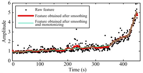
1) Moving average smoothing and monotonizing for the degradation features sequentially. Because we only care about the degradation trend of the system reflected by degradation features while excluding other details contained in the features, it is necessary to remove the baneful influence of noise or other external factors as possible. Through the above pretreatment, we can obtain the features which indicate the degradation trend of the system more intuitively. Fig. 1 illustrates the comparison between raw degradation features and the pretreated features.
Fig. 1Comparison between raw degradation features and the pretreated features
2) The following general prediction model is used to replace the previous specific model, which needs to be identified, to simplify the prediction process:
where is the degradation rate of the feature and defined as the ratio of the state at time to the state at the previous time . In general prediction model, the content of every particle is simplified and a particle includes only the state and the degradation rate , thus reducing computational complexity considerably. Moreover, we can compute real-time observations of in the iterative updating phase. It means that the resampling can be used in the estimation of , significantly reduce the influence of the initial distribution set of model parameters on prediction results.
3) The priori information of the degradation rate should be utilized completely. The degradation rate reflects the system degradation rate from the normal state to failure, and the estimation of determines the prediction of RUL for the system. Therefore, the accurate estimation for the evolution trend of degradation rate in the prediction phase is very important. Because the degradation behavior of equipment is a one-way variation over time, the range of the degradation rate after smoothing and monotonizing pretreatment is easily determined. According to the signification of degradation feature, a boundary or can be determined firstly. Another boundary can be obtained from the statistics of the extreme value of in historical data population. The distribution map of the degradation rate with different features is computed based on historical data statistics to guide the updating of particle state in the prediction phase.
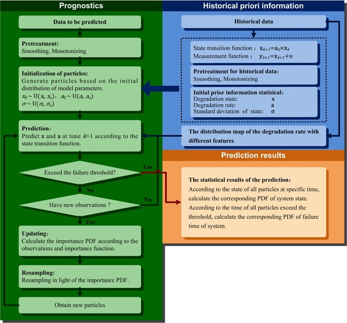
The flowchart of the DRT-PF prediction method is shown in Fig. 2.
Fig. 2Framework of the DRT-PF prediction algorithm
4. Case study and discussion
Rolling bearing is one of the most commonly used components in rotating machinery, and most of the failures of rotating machines are related to rolling bearing. Therefore, bearings can be considered as critical components because their failure significantly decreases availability and security of machines.
In the paper, a set of bearing acceleration degradation tests were conducted to verify the effectiveness of the proposed method. The experimental data came from the IEEE PHM 2012 Data Challenge organized by the IEEE Reliability Society and FEMTO-ST Institute [18].
As shown in Fig. 3, the experimentation platform is dedicated to test and validate bearings fault detection and diagnostic and prognostic approaches. A pneumatic jack, a vertical axis, and its lever arm and a clamp ring constitute the radial force generation unit, which can provide the maximum radial dynamic load of 4000 N. This makes bearing state deteriorate from normal state to failure in only several hours, thus providing real experimental data of characterizing the degradation of ball bearings in their whole service life (until the failure).
Fig. 3Test rig and the failure bearing
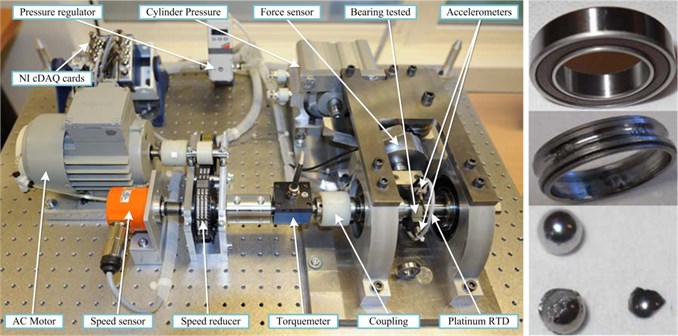
Characteristics of tested bearings: diameter of rolling elements 3.5 mm, number of rolling elements 13, diameter of the outer race 29.1 mm, diameter of inner race 22.1 mm, bearing mean diameter 25.6 mm.
Experimental operating conditions: rotation speed is 1800 r/min, the radial load is 4000 N, sampling frequency 25.6 Hz, sampled every 10 s, each sampling time is 0.1 s.
4.1. Extraction of degradation features
From the experimental data, we tried to extract different features in the time and frequency domains. However, neither the time domain features, such as root mean square (RMS), crest factor, and kurtosis of vibration signals, nor the frequency domain features, such as the magnitude at bearing defect frequencies, exhibited a consistent trend of bearing degradation. Therefore, according to the rating standard of vibration quality ISO 2372-1974, we selected the vibration intensity which combines the advantages of both time and frequency domain features as the degradation feature for RUL prediction [19]. The vibration intensity is defined as the RMS value of vibration velocity in the frequency range of 10-1000 Hz. It is a comprehensive description of equipment vibration and reflects the quantity of total vibrational energy including the energy of each harmonic. The vibration velocitycan be expressed as:
where is time length of the signal, is the vibration velocity of the object system. If the signal is discreet, Eq. (14) can be written as:
According to the properties of the Fourier transform, vibration intensity can be calculated in the frequency domain. For the vibration signal of points, the sampling frequency is , the vibration intensity can be calculated with DFT as:
The single-sided amplitude spectrum of vibration signal can be expressed as:
The corresponding frequency is:
The minimum integer greater than is denoted as . The maximum integer less than is denoted as . If is a vibration acceleration signal, then its vibration intensity in the frequency range of can be calculated as:
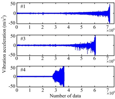
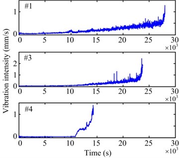
Fig. 4a) Raw vibration signals and b) their vibration intensities
a)
b)
The vibration intensity of some specific locations can be used as a criterion to judge whether equipment is operating normally. The vibration intensity is in a low level and stable state when the system is operating normally. Once fatigue damage or other faults occur at a certain component, the device enters a depletion phase and the fault will be reflected as the increase of vibrational energy. When vibration intensity increases to a certain extent, it will affect the operational safety of the system. Consequently, we can calculate the bearing vibration intensity with raw vibration data to obtain the degradation feature for RUL prediction.
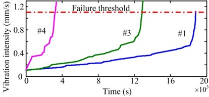
Among all the data, the vibration intensity of the data of three bearings (Bearing 1-1, 1-3 and 1-4, respectively referred to as #1, #3, and #4) exhibits a gradual degradation trend, as shown in Fig. 4. These three sets of data are chosen to verify the improved PF prediction method. With the three sets of data, a vibration intensity value of 0.1 mm/s was regarded as the initial point of the prediction and the failure threshold is set to be 1.1 mm/s. Then, through the pretreatment of smoothing and monotonizing, the final degradation features for PF prediction algorithm are obtained, as shown in Fig. 5.
Fig. 5Degradation features after pretreatment
4.2. Historical priori information
4.2.1. The initial distribution of parameters
Before the prediction, the initial distribution of the model parameters should be determined firstly. Particles are initialized with the uniform distribution. In the light of the Eq. (13), the parameters to be initialized include the degradation state , the standard variance of the state, and the degradation rate . In the iterative updating phase, resampling will be conducted for and . Therefore, their initial distribution can be set as an interval that is slightly larger than the range of historical inspection data. The standard variance can be calculated with the residual statistics between all raw features of historical data and the features of the pretreated data.
Because the prediction starting point is 0.1 mm/s, the initial distribution interval of the degradation state can be expressed as [0.08, 0.12], and the initial distribution interval of state standard variance is [0.005, 0.010]. The distribution intervals are obtained with the statistical results of three sets of data.
According to the definition of the degradation rate:
the degradation rates of degradation features for three sets of data are respectively calculated and the initial distribution interval of degradation rate can be obtained as [1.00, 1.03]. The initial distribution of all model parameters are shown in Table 1.
Table 1The initial distribution of model parameters
Model parameters | Uniform distribution boundary | |
Lower boundary | Upper boundary | |
0.08 | 0.12 | |
0.005 | 0.01 | |
1.00 | 1.03 | |
4.2.2. The distribution map of the degradation rate
Another work before prediction is the calculation of the distribution map of the degradation rate with different features. The distribution information will be used to guide the estimation of the degradation rate in the prediction phase. In the basic PF prediction method, degradation trajectory of all particles are extrapolated directly according to the updateded model parameters. During this process, a partcile would not be adjusted byany other ways, and the corresponding estimation errors of model parameters would accompany its evolution to the end. Whereas, DFT-PF needs specific degradation rate of the feature for extrapolating, that can control the accidental divergence of predictive error. It is not hard to obtain the distribution map of the degradation rate with different features. Firstly, the degradation rates of different historical data are assigned to the corresponding axis of the degradation feature, and then to calculate the degradation trend curve with the interpolation algorithm. Finally, the normal distribution of the degradation rate is fitted at each feature point and the distribution map of the degradation rate with different features is obtained and shown in Fig. 6. Different colors denote the dfferent values, and the bigger value indicate the more concentrated distribution.
Fig. 6The distribution map of the degradation rate with different features
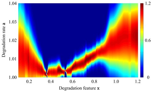
In Fig. 6, the distribution map can be roughly divided into three stages: (1) , the distribution of is relatively decentralized at the begining, but as the increase of , the distribution converges to a narrower range gradually. That is because the manifestations of different bearings differ widely at the early stage of faults, as severity deepening of faults, however, they would become stable. (2) , the distribution of always focuses on a narrow band. It means that the faults of bearings are in a stably degradation condition at this stage. (3) , distribution of becomes wider again, and expands like a funnel. It shows that, as long as the faults deteriorate to certain extent, the differences between different bearings or different faults become more and more obvious. Some of them would sped the deterioration until complete failure, while some others may retain previous level of degradation rate. Because of these complex situations during the degradation process of bearings, it is necessary to track the degradation rate for enhancing prediction performance.
According to Fig. 6, in the prediction phase, if degradation feature reaches 0.8, the corresponding degradation rate focuses on 1.010-1.015; and if reaches 1.0, the range of enlarges to about 1.01-1.03. We generate degradation rate values randomly based on the specific distribution obtained before, and substitute these values to prediction model for prediction of every particles at next step.
In addition, the guidance information for degradation rate prediction also includes the value range. According to the statistical results above, the value range of the degradation rate in the whole degradation process, except for a few outliers, is about [1, 1.04]. Through limiting the degradation rate with the algorithm, the particle divergence can be effectively controlled during the calculation.
4.3. Prognostic results and discussion
Some statistical priori information has been obtained with historical data and is helpful in predicting the degradation rate data of an individual sample. Because the details of every set of data are ignored in the obtained statistical priori information, three sets of data above also can be used to validate the method.
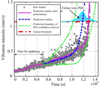
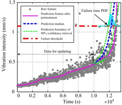
Fig. 7(a) depicts the prediction results of 500 observation points for #3 data. Because the relatively fewer data points are for model updating, the PDF range of RUL prediction is broad and the width of 90 % confidence interval is 3415 s. The error between the prediction median and the actual RUL is 770 s. The prediction results of 1000 observation points for #3 data are illustrated in Fig. 7(b). With the increase in the data points for updating, 90 % confidence interval range becomes smaller and the error between the prediction median and the actual RUL decreases to 550 s. In Fig. 7, the thick solid line denoting the prediction median has been traced to the nonlinear trend of the degradation feature. However, some great oscillations occur between 10000 s and 12000 s, causing a step jump of the degradation feature after pretreatment. Therefore, these details cannot be tracked and the prediction error becomes larger.
Fig. 7Prediction results of a) 500 and b) 1000 observation points for #3 data
a)
b)
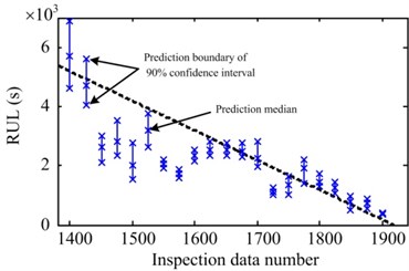
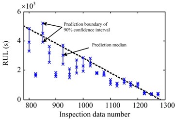
Fig. 8 illustrates the statistics of prediction results of various observation points. Fig. 8(a) shows the statistical prediction results for #1 data, which start from 1400 observation points. The RUL is predicted for every 25 points. The dotted line denotes the actual RUL curve and the asterisk line indicates 90 % confidence interval of RUL prediction at the corresponding time. The asterisk positions indicate the interval boundary and the prediction median. Like #1 data, in #3 data, the RUL is predicted for every 25 points from 800 observation points. The statistical results of the two sets of data are similar. Moreover, the errors between prediction results and the actual RUL gradually decrease with the increase of the known observations, while the prediction accuracy gradually increases. With the increase of observations, the width of the confidence interval becomes narrow, indicating that the prediction uncertainty gradually decreases. Moreover, the prediction results of these two sets of data tend to be lower than actual RUL. Because the oscillation at the initial stage of the raw feature is violent and its effect cannot be eliminated completely through pretreatment, prediction results are significantly lower than the actual value. However, the prediction result is very close to the actual RUL.
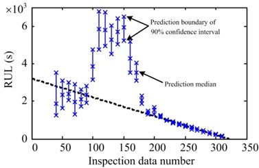
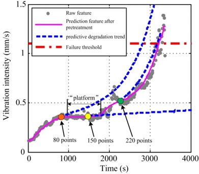
For #4 data, the prediction starts from 60 observation points and the RUL is predicted for every 10 points. The statistical results are shown in Fig. 8(c). Unlike #1 and #3 obviously, the results between 100 to 180 observation points greatly exceed the actual RUL. After that, the results converge to the actual RUL, and the corresponding confidence interval shrink to a very narrow range quickly. After that, the prediction and their variance are smooth and stable until the bearing failure. The reason caused this phenomenon is the particularity of #4 data, not the method itself. As shown in Fig. 9, the evolution trend ofthe degradation feature points of #4 data which less than 100 or more than 180, have better consistency with the diminishing trend of RUL, and compare with #1 and #3 data, they have better convergence and less fluctuation. But there is an 800 s “platform” phase of feature in the range of 100 to 180 points, which would produce a misleading effect on the calculation and cause prediction errors. When the inspection data number is in the range of the “platform”, such as 150 points, it is more reasonable to estimate that the degradation rate after would be close to the latest one. It means that current prediction results can not capture the turning point from the “platform” to ascending stage, so the predicted RUL is much more than actual RUL definitely. Obviously, this problem cannot be avoided in most of the prediction methods [14]. As long as the inspection data number is out of the “platform” period, the misleading effect disappeared. Moreover, because the prediction features after 2000 s retain a better level of convergence and consistency, so that all particles can rapidly converge to the actual RUL, the results become very satisfactory.
Fig. 8Prediction statistical result of a) #1, b) #3 and c) #4 data
a)
b)
c)
Compare with some traditional prediction approaches, particle filtering has more intuitive physical meaning, and could provide the crucial probability information of prediction results for decision maker. But for basic PF method, besides the shortcomings mentioned in Section 3.1, it lacks extra error control in the prediction phase. So it is usually powerless for the long-term prediction or other situations which prediction feature is dissatisfactory. During the experiment verification, we tried to process the same data with basic PF method. However much time is taken for determination of prediction model and initial distribution of model parameters, but we always can not obtain acceptable results, sometimes the particles are even no convergence. The proposed DRT-PF, through the dedicated pretreatment for degradation features, effectively improve their convergent behaviour and trend consistency, and effectively control the prediction error due to the strategy of degradation rate tracking. Though these measures can not fully remove the influences of the “platform”, they are important to optimize the degradation features extracted from vibration signal of bearings. From the case of #4 data, we can further determine the significance of the quality of degradation features to a prediction method. The good consistency between features and degradation trend of the component could ensure the accuracy of the results, and the convrgence of feature decide the convrgence of resultsin great degree. Therefore, in order to improve the ability of RUL prediction for mechanical components, besides improvement of method itself, trying to find a kind of more satisfactory prediction feature is equally important.
Fig. 9Analysis of predictive degradation trend for #4 data at different observation points
5. Conclusions
In the paper, we investigated the implementation process of the PF prediction method and pointed out a few shortcomings in detail. Aiming to these shortcomings, we proposed a novel DRT-PF prediction method, in which we improved the basic PF method from three aspects: the pretreatment of smoothing and monotonizing, the selection of general prediction model, and complete utilization of the useful information in historical data. Compared with the basic PF prediction method, the proposed method has the simplified implementation process and the better generality. In addition, the more historical data, the better prediction results would be. Then we utilized the accelerated whole life test data of rolling bearings to verify the effectiveness of the proposed method. The verification results show that the proposed method can be applied to predict the remaining useful life of rolling bearings.The further research will focus on how to find better degradation feature and improve the on-line prediction performance based on the DRT-PF framework.
References
-
Kruzic J. J. Predicting fatigue failures. Science, Vol. 325, 2009, p. 156-157.
-
Yogesh G. B., Ibrahim Z., Sagar V. K. Overview of remaining useful life methodologies. ASME 2008 International Design Engineering Technical Conferences and Computers and Information in Engineering Conference, American Society of Mechanical Engineers, New York, ASME, 2008, p. 1391-1400.
-
Shao Y., Nezu K. Prognosis of remaining bearing life using neural networks. Proceedings of the Institution of Mechanical Engineers, Part I: Journal of Systems and Control Engineering, Vol. 214, Issue 3, 2000, p. 217-230.
-
Lee J. A similarity-based prognostics approach for remaining useful life estimation of engineered systems. IEEE International Conference on Prognostics and Health Management, Denver, 2008, p. 1-6.
-
Dong M., He D. A segmental hidden semi-Markov model-based diagnostics and prognostics framework and methodology. Mechanical Systems and Signal Processing, Vol. 21, Issue 5, 2007, p. 2248-2266.
-
Di Maio F., Tsui K. L., Zio E. Combining relevance vector machines and exponential regression for bearing residual life estimation. Mechanical Systems and Signal Processing, Vol. 31, 2012, p. 405-427.
-
Li C. J., Lee H. Gear fatigue crack prognosis using embedded model, gear dynamic model and fracture mechanics. Mechanical Systems and Signal Processing, Vol. 19, Issue 4, 2005, p. 836-849.
-
Feng Z., Zuo M. J., Chu F. Application of regularization dimension to gear damage assessment. Mechanical Systems and Signal Processing, Vol. 24, 2010, p. 1081-1098.
-
Orchard M. E. A Particle Filtering-Based Framework for On-Line Fault Diagnosis and Failure Prognosis. Dissertation for the Doctoral Degree, Atlanta, Georgia Institute of Technology, 2007.
-
Zio E., Peloni G. Particle filtering prognostic estimation of the remaining useful life of nonlinear components. Reliability Engineering and System Safety, Vol. 96, Issue 3, 20011, p. 403-409.
-
Jin G., Matthews D. E., Zhou Z. A Bayesian framework for on-line degradation assessment and residual life prediction of secondary batteries in spacecraft. Reliability Engineering and System Safety, Vol. 113, 2013, p. 7-20.
-
Saha B., Goebel K. Uncertainty management for diagnostics and prognosticsof batteries using bayesian techniques. IEEE Aerospace Conference, 2008, p. 1-8.
-
He W., Williard N., Osterman M., Pecht M. Prognostics of lithium-ion based on Dempster-Shafer theory and the Bayesian Monte Carlo method. Journal of Power Sources, Vol. 196, 2011, p. 10134-10321.
-
Chen C., Pecht M. Prognostics of lithium-ion batteries using model-based and data-driven methods. IEEE International Conference on Prognostics and Health Management, Denver, 2012, p. 1-6.
-
Wang D., Miao Q., Pecht M. Prognostics of lithium-ion batteries based on relevance vectors and a conditional three-parameter capacity degradation model. Journal of Power Sources, Vol. 239, 2013, p. 253-264.
-
Gordon N. J., Salmond D. J., Smith A. F. M. Novel approach to nonlinear/non-gaussianbayesian state estimation. IEE Proceedings on F Radar and Signal Processing, Vol. 140, Issue 2, 1993, p. 107-113.
-
Carpenter J., Clifford P., Fearnhead P. Improved particle filter for nonlinear problems. IEE Proceedings on Radar, Sonar and Navigation, Vol. 146, Issue 1, 1999, p. 2-7.
-
http://www.femto-st.fr/en/Research-departments/AS2M/Research-groups/PHM/IEEE-PHM-2012-Datachallenge.php.
-
Fan X. H., An G., Wang K., Wu D. M. Research on vibration severity for machine condition monitoring. Journal of Academy of Armored Force Engineering, Vol. 22, Issue 4, 2008, p. 46-49, (in Chinese).
About this article

This work was supported by the National Natural Science Foundation of China (Grant Nos. 51105366 and 51475463) and the Research Project of National University of Defense Technology. Additionally, the authors would like to thank the IEEE Reliability Society and FEMTO-ST institute, for sharing the experimental data.
