Shift invariant sparse coding ensemble and its application in rolling bearing fault diagnosis

2.1. Introduction of SISC

In the theory of SISC [9], by using an over complete dictionary matrix $\left[{\mathbf{d}}_1,{\mathbf{d}}_2,\cdots ,{\mathbf{d}}_M\right]\in {\mathbb{R}}^{Q\times M}$ which contains $M$ prototype bases for columns, a signal ${\mathbf{s}}_k\in {\mathbb{R}}^N$ can be represented as the sum of the convolutions of these bases and coefficients:

where $\mathrm{*}$ indicates convolution, coding coefficient ${\mathbf{x}}_{m,k}\in {\mathbb{R}}^P$ is sparse, $\mathbf{\epsilon }$ is a normalized Gaussian noise, $Q<N$, $P<N$, and $Q+P-1=N$.

To make the optimization convex, the basis ${\mathbf{d}}_m$ and coefficient ${\mathbf{x}}_{m,k}$ are optimized repeatedly. The cost function for evaluating the representation of the signal set containing $K$ signals is as follows [14]:

where ${‖\cdot ‖}_2$ is $l^2$ norm, $\beta$ is a parameter, which determines the degree of sparsity. The basis ${\mathbf{d}}_m$ needs to be normalized, namely ${‖{\mathbf{d}}_m‖}_2^2=\text{1}$. If ${\mathbf{d}}_m$ and ${\mathbf{x}}_{m,k}$ are solved at the same time, then the optimization problem is no-convex, making it more difficult to get a stable and convergent solution. As a result, the basis ${\mathbf{d}}_m$ and coefficient ${\mathbf{x}}_{m,k}$ are optimized iteratively and repeatedly according to the maximum posterior probability estimation until convergence. Many experiments have validated this approach as highly effective [4]. Many scholars have studied how to solve and simplify this problem. Smith [9] and Blumensath [8] proposed the most common optimization procedure. They directly updated the bases based on gradients, and successfully employed this way in voice and music processing. Grosse [14] and Tang [11] transformed signals into frequency domain, and used the gradients to solve the optimal bases. The gradient-based SISC (GSISC) method by Smith and Blumensath is as follows:

Let ${\mathbf{e}}_k={\mathbf{s}}_k-\sum _{m=1}^M{\mathbf{d}}_m*{\mathbf{x}}_{m,k}$, the derivation of a given cost function $\psi \left(\theta \right)$ with respect to the $q$th element of basis ${\mathbf{d}}_m$ is [8, 9]:

where $\text{1}\le n\le N$, $\text{1}\le n-q+\text{1}\le P$, $\text{1}\le k\le K$.

Similarly, the derivation of a given cost function $\psi \left(\theta \right)$ with respect to the $p$th element of coefficient vector ${\mathbf{x}}_{m,k}\left(p\right)$ is as [8, 9]:

where $\text{1}\le q+p-1\le N$, $\text{1}\le q\le Q$.

After using the gradients in Eq. (3) and (4) to optimize the bases and coefficients iteratively until convergence is reached, the original signals can be sparsely represented by learned bases and coefficients. Besides, the coding coefficients could be also solved by OMP, FOCUSS algorithm, etc. As outlined above, the gradients used in these optimization algorithms are estimated through the numerical difference, and so the exact step length per iteration is hard to be taken, and the best evaluation in each iteration shall not guaranteed.

2.2. The procedure of ISISC

The efficient K-SVD algorithm [4] updates the bases one by one, rather than all at once. Inspired by this idea, the bases of ISISC are also updated one by one in the dictionary learning process. First, due to the sparsity of coefficients, the nonzero coefficients are extracted to markedly reduce the scale of the optimization problem. Then, the convolution problem is converted into a small scale symmetric positive linear equation, which can be directly solved by Cholesky algorithm without being influenced by former iterative result. So this scheme converges faster than GSISC. In the coefficient update stage, higher efficiency is achieved by the employment of OMP, fast convolution algorithm and extraction of only nonzero coefficients.

2.3. SISC ensemble for pattern recognition

Sparse coding and pattern recognition have natural relationship [6]. Under the limitation of sparsity, the most closely related basis with the original signal will be automatically selected, and the other bases are refused. The robustness and accuracy of sparse coding for pattern recognition have been validated in the field of face recognition and voice processing. The original dictionary can be constructed directly by selecting some training samples, and can be learned through dictionary learning algorithm. Dictionary learning [5] is able to learn the internal structures and main features of original signals through a group of sparse bases, and it is insensitive to Gaussian noise. In this paper, the ISISC proposed in Section 2.2 is used for dictionary learning, and one sub dictionary per class is learned.

In this investigation, the sub dictionaries are not combined together in order to avoid destroying the structure of each sub dictionary. But under the same sparsity of $T_0$, each sub dictionary is employed respectively for sparse representation. When the label of the sample and the label of the sub dictionary are the same, the reconstruction error should be the lowest, which means that the label of the dictionary with lowest reconstruction error is expected to be the label of the sample.

Unfortunately, real-world vibration signals are often contaminated by a lot of noise, and the number of available training sample is limited. Thus it is necessary to further improve the classification ability of sparse coding. Some scholars added distinctive constraints to sparsity when training dictionary so that the dictionaries can be more discerning. However, this approach will increases the difficulty of optimization and make some fast algorithm potentially unable to work well, or even make convergence unstable. Ensemble learning introduced in recent years is a very powerful machine learning method [12]. It synthesizes a few different classifiers, and can get better performance than the individual classifier that composes it. AdaBoost algorithm [13], proposed by Freund and Schapire, is a valid approach to ensemble learning. The same group of training samples are used, but the weights of samples are adaptively changed after a classifier is trained. Therefore, the error sample will be paid more attention by the next classifier. Lastly the combination of classifiers, whose individual decisions are weighted by voting, will exhibit better performance. It has been verified that when the error of individual classifier is lower than 50 %, the error of combination will descend exponentially close to zero [13].

Although the sparse coding is not the same as conventional classifiers, the increase in the weight of an error sample will enhance its ability to recognize the pattern of a sample. The rise of a sample’s weight will result in the fact that the structure of the sub-dictionary learned is closer to the error sample. That is to say, the dictionary has superior ability to represent this sample, while keeping other sub-dictionaries representative ability unchanged. Therefore the reconstruction error of the sample by the new weighted sub-dictionary is relatively decreased, and the probability of being categorized as required is increased. The algorithm of ISISC ensemble is presented in Table 1 [18].

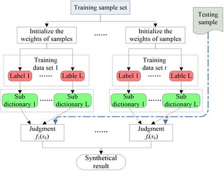
This paper fused the AdaBoost algorithm into ISISC to enhance the successful rate for recognition faults, and the diagnostic procedure is shown in Fig. 1. The signals under different loads have diverse energies. By normalizing them, it is able to guarantee that the relative weights of samples are identical. The sub-dictionary is trained by ISISC, one for each class, in sequence according to the labels. After the first classifier was trained, and the weights of all training samples are then updated according to the method demonstrated in Table 1. Subsequently the sub-dictionaries of the next classifier are trained. Following this way, all the ISISC classifiers are to be trained. For an unlabeled sample, firstly, it is to be reconstructed under sparsity $T_0$ respectively by using each sub dictionary of the first classifier; secondly, it is to be classified based on the minimum reconstruction error. In such way, the sample is identified by all the ISISC classifiers. Eventually all the decisions are synthesized for the final judgment in the light of the weighted algorithm in Table 1.

Fig. 1ISISC ensemble procedure

3.1. Comparison between ISISC and GSISC

A simulated pulse sequence of vibration signal caused by a single point defect on rolling bearing is as follows:

where $t$ is time, $y\left(t\right)$ has a damped sinusoids function and its amplitude is modulated by a sinusoids function. $i$ is the count number of pulses, ${\tau }_i$ is the beginning time of pulse. Here ${\tau }_i$ is set as a random number in order to test the adaptability of SISC. $T$ is the period of the pulses, and here it equals 120 points. The attached noise is Gaussian noise, and its signal to noise ratio (SNR) is –2 dB. $y\left(t\right)=e^{pt}\mathrm{s}\mathrm{i}\mathrm{n}\left(2\pi f_{b}t\right)$ is a pulse resonance induced by the single point defect, and it is normalized in this study. $p=\text{1200}$ is the damping coefficient, and $f$ is oscillation frequency, which indicates the damped natural frequency of the system.

The signal has 10240 points, and it is averagely separated into ten samples. GSISC and ISISC are respectively used to represent the signal set for comparison. The length of a basis is set as 60 points, and only one basis is learned. For GSISC optimization, the conjugate gradient method is chosen, and the step length is determined by both the golden section search and parabolic interpolation. The sparsity is set as 9 in ISISC, and the online learning algorithm is not adopted in this experiment.

The convergence curves of residual energy is shown in Fig. 2. The original basis, the bases learned by ISISC and GSISC are illustrated in Fig. 3. ISISC converges to the optimal solution within a few iterations, and its learned basis resembles the original pulse resonance. Yet, GSISC converges considerably slowly, and its solution is slightly worse than that of ISISC. Moreover, there is a little distortion with its learned basis.

Fig. 2Residual energy

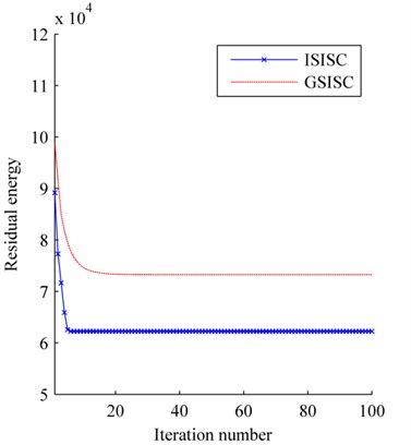
Fig. 3Bases: a) origin, b) ISISC, c) GSISC

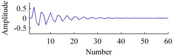
a)

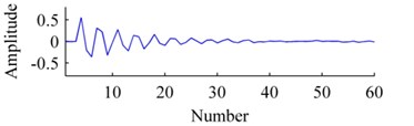
b)

c)

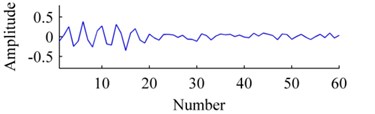
Fig. 4The signal: a) origin, b) added with noises, c) ISISC, d) GSISC

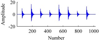
a)

b)

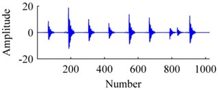
c)

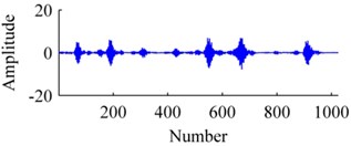
d)

Fig. 4 displays an original sample, and corresponding reconstructions by ISISC, GSISC. The signal is seriously contaminated by noises, but ISISC still excellently recovers it. Unlike ISISC, the reconstruction of GSISC distorts and contains a few noises, and the peaks of pulses are not well preserved.

To comprehensively appraise the performances of these two algorithms, the original signals are mounted with noises of different SNR values. The SNR and MSE values of the 100th iteration are applied for evaluation. Fig. 5 shows the average results of ten times. No matter how many noises added to the original signals, ISISC always outperforms GSISC in both SNR and MSE. In contrast to GSISC and in consideration of the new dictionary updated algorithm and the experiment, ISISC is more efficient, exhibits faster convergence, is not as easy to fall into local optima, and has higher probability to find better optimal solution.

3.2. Application of ISISC ensemble to mechanical fault diagnosis

Rolling bearing is one of the most widely used elements in machinery, and its status is vital to the whole system. The database used in this paper is obtained from the Case Western Reserve University Bearing Data Center [19], which is considered as a benchmark for machinery diagnosis. Single point faults with diameters of 0.007, 0.014, 0.021 and 0.028 inches (1 inch$=$2.54 cm) are introduced separately at the outer race (at 6:00 directions), inner race and ball. Tests are carried out respectively under loads of 0, 1, 2, 3 hp (1 hp $=$ 746 W), with corresponding shaft speed being 1797, 1772, 1750, 1730 rpm. The sampling frequency is 12 kHz. In order to determine the location and the severity of the fault, the data are divided into 10 classes, and each class contains four data with the loads of 0, 1, 2, 3 hp. The relationship between labels and data is shown in Table 2. Normal indicates the bearing is Normal. IR, B and OR respectively represent the inner race fault, ball fault and outer race fault. The number followed suggests the fault severity. For example, OR007 represents the outer race of the bearing is fault, and the fault diameter is 0.007 inch.

Fig. 5The performances of ISISC and GSISC with different noises

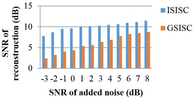
a) SNR of reconstruction

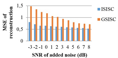
b) MSE of reconstruction

Every data is truncated into time-series with a 2048-point window block. About 118 samples are generated from each data of normal condition, while each data under faulty condition contains approximately 59 samples. The ISISC ensemble proposes in this report is used to train and test the data. The number of classifiers in ensemble is five; each sub dictionary for one class $T_0$ contains 15 bases, and the sparsity is 26. The length of a basis is 150 points, and as its length will contain about 2 pulses in one basis, the basis will include not only the underlying information of resonance but also the fault feature frequency of each condition.

Liu [10] has applied this data set, employed SISC for feature extraction, and designed a linear classifier for identification. In his experiment, all the samples are smoothed for pre-processing. For the purpose of confirming the advantage of ISISC ensemble, two similar experiments are conducted. In the first experiment, 20 samples per data under every load are randomly selected as training set, and all the samples in the database are tested. This experiment is implemented by ISISC ensemble. The single ISISC classifier is also tested, only using 25 samples per each data for training. In Liu’s experiment [10], half samples in each data are trained which is more than either ISISC ensemble or ISISC classifier. The average accuracy rate of 0-3 hp for each class is shown in Fig. 6.

Although ISISC ensemble uses the least training samples, its success rates are highest and stable in general. This demonstrates that ISISC ensemble can accurately determine the condition of bearing as well as fault severity. Moreover, ISISC classifier and ISISC ensemble both perform better than Liu’s method on the whole. Apart from that, the efficiency has been markedly improved. Using a laptop with a dual-core 2.2 GHz CPU and DDR 667 2G memory, the training time of one class using Liu’s method is approximately one hour, whereas the time of ISISC ensemble is about ten minutes and the time of ISISC classifier is as few as 2 minutes. In comparison with Liu’s method of adding a classifier for recognition and pre-processing the samples, all the samples can be directly put into ISISC ensemble for fault recognition without any people’s operation. Dong [20] employed principal components analysis to extract features which were input into Morlet kernel support vector machine for classification. He recognized the same data of Normal, IR007, IR014, IR021 and IR028, with the accuracy rates are all as high as 100 % under the best parameters. By contrast, the accuracy rates of these data using ISISC ensemble are also 100 %, but the classes of ISISC ensemble are 10 which is more than that of Dong’s experiment.

Fig. 6The average accuracy rate of 0-3 hp for each class

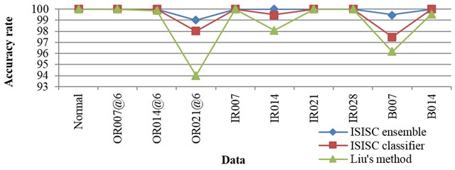
Fig. 7The accuracy rates of each data under 0-3 hp

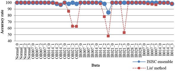
When the rolling bearing is running, its load frequently varies. The rolling bearing can hardly run at an accurate speed, and the speed usually varies in a small range. Therefore, the monitoring system needs to be robust enough against the alteration of load and the variation of speed within a small range. So another experiment is done, with only the data under 0 hp selected for training and the corresponding speed being 1797 rpm. In the training set, 50 samples per class are randomly chosen. All the data are selected for testing, namely all the data under 0, 1, 2, 3 hp, and corresponding speeds are 1797, 1772, 1750, 1730 rpm respectively. Liu [10] has also done the similar experiment, and the results of our experiment together with those of Liu’s are listed in detail in Fig. 7. The accuracy rates of ISISC ensemble are higher than Liu’s for all the data. The worst one of our method is above 80 %, while Liu’s worst rate is below 50 %, so the stability of ISISC ensemble is stronger. Zhu [2] has applied K-SVD based on envelope spectrum to do similar experiment, but he’s algorithm need to re-sample the data, so it was not robust enough to speed.

As mentioned above, it is evident that ISISC ensemble is more accurate than other methods. Apart from that, the most outstanding advantage of ISISC ensemble is that it lessens people’s participation and is much easy for application. The signal pre-processing, feature extraction and pattern recognize are not needed in this algorithm, and all the learning processes are implemented by computer itself. ISISC ensemble can still make precise judgment even when the load varies or the speed changes in a certain range.