Abstract
For the system degradation process undergoing a sudden change, optimal maintenance policies were developed using the cumulative damage model and two-stage degradation modeling. Single shock damage value and the number of shock times are assumed to be normal distribution and homogeneous Poisson process, respectively. On this basis, average long-run cost rate of a renewal cycle was modeled with considering the probabilities of corrective, preventive and continuous monitoring, respectively. In order to develop an optimal policy, four types of maintenance policies (i.e., global, time-depended, adaptive and simplified adaptive policies) were analyzed with different alarm thresholds and inter-inspection time. Influence analysis of different parameters for maintenance policy was given, where different maintenance policies were compared in terms of average long-run cost rate. In addition, the impacts of degradation model parameters (i.e., change-point distribution, shock strength, shock frequency) on the average long-run cost rate were analyzed. Finally, maintenance policy for gearbox degradation experiment was analyzed in case study.
1. Introduction
Performance degradation is a common phenomenon in many systems, especially in mechanical and structural systems. Deterioration modeling plays a more and more important role in maintenance decision-making. Many researchers have mainly studied intensively systems degradation with stationary processes to optimize maintenance problems [1-4]. However, the degradation processes for many systems are non-stationary due to internal mechanism or external environment influences etc. [5]. For example, some systems are deteriorating in a process of two stages [5-11], where the degradation rate is usually small in the first stage and large in the second stage.
In order to study system degradation, it is necessary to establish corresponding degradation model. The deterioration process model with independent random increment is divided into two types, continuous time model and cumulative damage model. The continuous time model [12, 13, 14] presents system degradation in terms of continuous time stochastic process. The most representative models for continuous time model are Brownian motion model and Gamma process model. Whereas, in the cumulative damage model [15, 16, 17], it is assumed that system degradation process is discrete. The model describes the degradation process by cumulating a number of random increments caused by damage in the system operation. Existing studies for two-stage degraded system mainly focused on continuous time model. Application of cumulative damage model to two-stage degradation process was seldom investigated.
Due to the discrepancy of different deterioration modes for a two-stage degraded system, maintenance decision-making methods for single-stage degradation process system cannot be applied to two-stage deteriorating mode system. In order to solve the problem, In order to solve the problem, studies have been done and a number of maintenance strategies were developed. An activation zone method for maintenance decision-making is presented by Saassouh [6] with considering the random change of degradation rate, but the degradation rate change time is assumed to be continuous and perfectly monitored. Ponchet [12] developed two maintenance decision-making methods with and without considering the deterioration mode change in system degradation processes, respectively. The results of numerical example show that it can bring considerable benefits if a policy with changeable thresholds was used. A predictive maintenance policy for a system with two deterioration mode based on process data was proposed by Zhao [18], and the maintenance actions were implemented based on different reliability thresholds. Some maintenance policies for two-stage deteriorating mode systems have been presented, but no much study has been done to investigate the performance of different maintenance polices with different thresholds and inspection intervals.
In this paper, degradation modeling and maintenance decision-making methods for two-stage deteriorating mode system based on cumulative damage model will be investigated. The main contributions of this study are: (a) Cumulative damage model is used for two-stage degradation modeling, and it shows system degradation rate change through different shock strengths and shock frequencies. (b) An optimal policy of a two-stage degraded system is developed by analyzing and comparing four types of maintenance policies (global, time-depended, adaptive, simplified adaptive).
The remainder of this paper is organized as follows. Section 2 is devoted to two-stage deteriorating modeling based on cumulative damage model. Section 3 studies four kinds of maintenance policies and analyzes maintenance policy evaluation method. Numerical examples are used to analyze the influence of different factors on maintenance policies in Section 4. Conclusions are made in Section 5.
2. Two-stage deteriorating modeling
2.1. System description
The considered system is assumed to be an observable system which degrading stochastically. The degradation level at time is supposed to be presented by a random variable [19, 20]. The system degradation process is an increasing stochastic process with initial state . System will be declared as failed when deterioration level exceeds a failure threshold (namely ). is defined as system failure time. System failed does not mean that the system cannot work, but implies that it’s economic and safety impacts will be unacceptable if it still in operation.
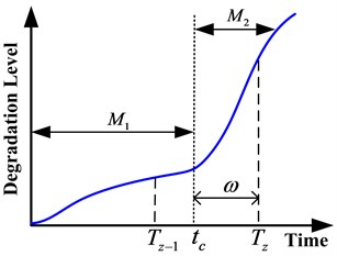
Fig. 1Two-stage degradation process
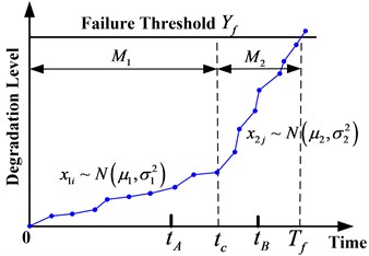
System degradation rate changes at time during a life cycle (as shown in Fig. 1). It means that the parameters of system degradation process undergo transitions at change-point . The system is supposed to be in a nominal degradation mode and denoted by before . After , the system degradation mode evolves to an accelerated mode . Degradation rate is usually small in the first stage and large in the second stage . Therefore, system degradation process can be modeled by two stochastic processes under the same law but with different parameters [6].
Most physical degradation observation and the property of the Levy processes have shown that system deterioration can be thought as the accumulation of large numbers of small shocks [21], and deterioration level can be defined as the sum of damage values due to shock. When the system is in mode , damage values ( 1, 2; 0, 1, 2, …) are assumed to be normally distribution, . is a constant in mode (see Fig. 1). Random variable represents the number of shock times during time [0, ] and it obeys to homogeneous Poisson distribution with strength in mode . Therefore, the probability of shock times just as in mode is:
For the convenience of expression, in this paper is denoted as shock strength and is denoted as shock frequency. It is not difficult to find that shock strength and shock frequency decide the size of degradation rate.
2.2. Degradation level modeling
In the two-stage degradation process, the value of damage time may be in the first stage () or in the second stage (). The calculation methods of degradation level are not alike in different degradation stage. According to the above notation, degradation level at time can be written as:
where stands for degradation level in mode , if is true and otherwise. When , the degradation level is:
In this case, the probability of shock times equal to within time [0, ] is the same to Eq. (1). Due to every shock damage is independently and unrelated, it can be known from the characters of normal distribution (the sum of normal distribution parameters still in line with normal distribution) that is obey to normal distribution, namely:
When , degradation level consists of the damage in first stage and the damage in second stage . In this case, degradation time length in the first stage is , to the second stage. Hence, the system degradation level is:
Similar to the Eq. (4), system degradation level is in line with normal distribution, there is:
Because shocks between the two stages are independently, the probability of the number of shock times just as in mode and equal to in mode is:
2.3. Reliability modeling
In engineering practice, the change-point for degradation rate is not fixed, but is distributed in a certain time interval. Shown as Fig. 1, the time distribution interval of change-point for degradation rate is [, ], in other words, the deteriorating mode may change at any time from to when system works during time [, ].
System reliability is the probability for degradation level less than failure threshold when damage time is . Shock strength, shock frequency and change-point should be considered in reliability modeling, which are main factors in cumulative damage model. Reliability modeling for two-stage degraded system is specific expressed as following.
When , system reliability is:
When , system reliability is:
where is the probability density distribution function for change-point during time [, ].
3. Maintenance policies
Research of maintenance decision-making is one of the focuses for system degradation modeling. Condition-based maintenance policy widely uses in various systems, which is structured according to the information available through on-line monitoring [12]. In order to reduce maintenance costs, preventive maintenance actions take place before system failure by monitoring. In other words, suitable monitoring method and maintenance policy can help to improve the efficiency and profitability of a system.
The selections of alarm threshold and inter-inspection time are the keys to maintenance policy. According to different alarm thresholds and inter-inspection times, this paper considers four kinds of maintenance decision-making methods. The first kind of method is global maintenance policy. There are just one alarm threshold and one inter-inspection time in this method, which are constants and never change. The second kind of method is time-depended maintenance policy. There are also one alarm threshold and one inter-inspection time in this method, but the inter-inspection time is change with system working time. The next kind of method is adaptive maintenance policy. Different alarm thresholds and inter-inspection times corresponding to different degradation rates, that is say, there are two alarm thresholds and two inter-inspection times in this method. The finally kind of method is simplified adaptive maintenance policy. This method is similar to adaptive maintenance policy, but it just has one inter-inspection time.
In the framework of this study, there are three possible maintenance actions, inspection, preventive maintenance and corrective maintenance, respectively. System is perfectly monitored through periodic monitor, and system state restores to be as good as new after preventive maintenance or corrective maintenance with negligible time.
3.1. Global maintenance policy
In order to show the importance of considering the changes of system degradation rate, traditional maintenance decision-making method is presented in the first place, which called global maintenance policy. The method just defines a single alarm threshold and a single inter-inspection time , as done in Dieulle et al. [22]. It is not difficult to find that the method only pay attention to system degradation level and ignore the degradation rate.
The possible maintenance actions which can put into practice after inspection time are defined as follows:
• If , do nothing and the system is left as it is until next inspection time .
• If , the system is too badly deteriorated so it is necessary to perform preventive maintenance.
• If , the system is considered as failed and it has to be performed corrective maintenance.
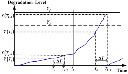
The rule of global maintenance policy is illustrated in Fig. 2.
Fig. 2Global maintenance policy
3.2. Time-depended maintenance policy
As the degradation rate in mode larger than in mode , the inter-inspection time should be shorter and shorter in term of work time. This kind of maintenance decision-making method called time-depended maintenance policy. For example, the inter-inspection time of th monitor is , the next inter-inspection time is , and .
The possible maintenance actions which can put into practice after inspection time are defined as follows:
• If , do nothing and the system is left as it is until next inspection time .
• If , the system is too badly deteriorated so it is necessary to perform preventive maintenance.
• If , the system is considered as failed and it has to be performed corrective maintenance.
The rule of time-depended maintenance policy is illustrated in Fig. 3.
Fig. 3Time-depended maintenance policy
3.3. Adaptive maintenance policy
According to the characteristics of system degradation rate suddenly changes from nominal mode to accelerated mode , Saassouh et al. [6, 12] put forward adaptive maintenance policy. The method is different with global maintenance policy, it considers system degradation level and degradation rate. As a result, this maintenance decision-making method is more responsive to systems with two-stage deteriorating mode.
The alarm threshold and inter-inspection time for adaptive maintenance policy are defined as follows:
Set as the alarm threshold and is the inter-inspection time for nominal degradation mode . When the inspection time is less than change-point (), the possible maintenance actions which can put into practice are defined as follows:
• If , do nothing and the system is left as it is until next inspection time .
• If , the system is too badly deteriorated so it is necessary to perform preventive maintenance.
• If , the system is considered as failed and it has to be performed corrective maintenance.
Set as the alarm threshold and is the inter-inspection time for accelerated degradation mode . When the inspection time is greater than change-point (), the possible maintenance actions which can put into practice are defined as follows:
• If , do nothing and the system is left as it is until next inspection time .
• If , the system is too badly deteriorated so it is necessary to perform preventive maintenance.
• If , the system is considered as failed and it has to be performed corrective maintenance.
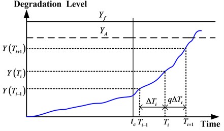
As the degradation rate for mode is greater than mode , so the maintenance policy parameters and . The rule of adaptive maintenance policy is illustrated in Fig. 4.
Fig. 4Adaptive maintenance policy
3.4. Simplified adaptive maintenance policy
Adaptive maintenance policy so complex that not suitable for engineering application. Therefore, adaptive maintenance policy is simplified in application by some researchers [12]. Inter-inspection time is a constant value and never changes in simplified adaptive maintenance policy.
The maintenance policy rule (alarm threshold, possible maintenance action) is similar to adaptive maintenance policy, the only difference is that: no matter or , the next inspection time always (namely ).
3.5. Maintenance policy evaluation
3.5.1. Evaluation method
Maintenance cost occurs when a maintenance action is performed. In this study the average long-run cost rate over an infinite time span is used to evaluate maintenance policy. As it has assumed that system state restores to as good as new if a preventive/corrective maintenance action performed, renewal reward theory [23] can be used to calculate the average long-run cost rate as follows:
where is the total maintenance cost at time , is the average time length of a renewal cycle.
The total maintenance cost in a renewal cycle can be expressed as follows:
The expected time length of a renewal cycle is written as:
Adaptive maintenance policy is the most complex method relative to other three maintenance policies, which parameters obtained more difficult. In this paper, parameters obtained method of adaptive maintenance policy are mainly analyzed, parameters for other three maintenance policy can also be obtained as this method.
3.5.2. Probability of corrective maintenance
If any one event of the following events (, , ) occurs, system is considered as failure. That is to say, system needs corrective replacement and it will cause corrective maintenance cost . Take the event as a example, system degradation process is in stage (), if the degradation level for th inspection and for th inspection, corrective maintenance action will be performed.
The probability for a corrective maintenance in a renewal cycle is expressed as:
System cumulative damage distribution is the probability for system degradation level less than a certain value when shock time is . The formula of cumulative damage distribution in stage can be denoted as:
Therefore, the density function of cumulative damage distribution in stage is:
The specific analytic formula of the probability for corrective maintenance event is expressed as follows:
where, is the probability of the number of shock times just as during time , is the probability of the number of shock times equal to within time , is the probability for system degradation in the first stage .
The probability for corrective maintenance events , can be expresses as follows:
3.5.3. Probability of preventive maintenance
If any one event of the following events (, , ) occurs, it is considered that preventive replacement needs to be performed and it will cause preventive maintenance cost . When a twice continuous monitoring just happened before and after the change-point for degradation rate (), if the degradation level for ()th inspection and for th inspection, preventive maintenance action will be performed.
The probability for a preventive maintenance in a renewal cycle is expressed as:
The probability for preventive maintenance events , , can be written as follows:
3.5.4. Probability of continuous monitoring
If any one event of the following events (, ) occurs, the system is left as it is until next inspection time and it will cause monitoring cost .
The probability for system left until next inspection in a renewal cycle can be expressed as:
The probability for continuous monitoring events , can be written as follows:
Average number of monitoring actions in a renewal cycle is:
3.5.5. Expected time length of renewal cycle
As Eq. (14) shown, expected time length of renewal cycle is affected by system life and average work time length when system ends with preventive replacement. If system faults, it is considered that system will not work any time. Therefore, the expected time length when system ends with corrective maintenance is the time interval for degradation level from initial value 0 to failure threshold . However, the expected time length when system ends with preventive maintenance is different. System will no longer work if monitoring shows preventive replacement should be performed, so system life when system ends with preventive maintenance is times of inter-inspection time .
System fault occurs in the second stage when system degradation with two-stage mode. System life is affected by shock strength , and change-point . The system mean time to failure is:
The average system life when system ends with preventive maintenance is:
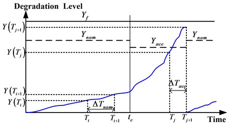
Fig. 5The definition of ω
Where is the number of monitoring in mode for event , is the number of monitoring in mode for event , the time length from to next inspection time is (as shown in Fig. 5), is the distribution density function of w during [, ].
4. Influence analysis of different parameters for maintenance policy
This section aims to find some characteristics for two-stage deteriorating mode system: (a) Making a comparison of the average long-run cost rate for different maintenance policies in the same situation in order to raise the awareness of monitoring method. (b) Studying the influence of parameters in the degradation model and average long-run cost model, for the purpose of improving the understanding in two-stage deteriorating modeling and developing an optimal maintenance policy.
4.1. Choice of parameters values
In this study, the time distribution of change-point is assumed to follow uniform distribution. In order to emphasize the influence of distribution of change-point , different uniform distribution parameters are considered as follows:
• Change-point of two-stage degradation mode: .
• Early change-point of two-stage degradation mode: .
• Middle change-point of two-stage degradation mode: .
• Late change-point of two-stage degradation mode: .
The upper limit of change-point distribution 200 is considered that a majority of system failures occur in degradation mode and seldom in degradation mode . Early and late time distributions present the first and second half of full change-point distribution, respectively.
In order to make the influence analysis of different parameters more close to the actual situation of gearbox degradation process, the selection of failure threshold is based on the actual value of gearbox life-cycle experiment in Section 5. Therefore, the failure threshold is evaluated as 10000 g2 in this study. Meanwhile, for the purpose of ensuring the credibility of optimization results for global maintenance policy (the optimization results will be regarded as a basis of comparison), the unit maintenance costs are evaluated as other literatures [1, 12, 24], so = 5, = 50, = 100.
4.2. Influence of maintenance policy
Fig. 6EC∞ is affected by adaptive maintenance policy parameters
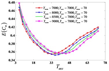
a) is affected by and
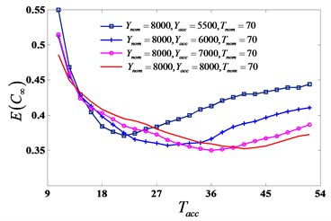
b) is affected by and
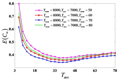
c) is affected by and
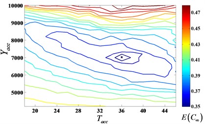
For the purpose of studying on the influence of different monitoring methods, the four kinds of condition-based maintenance policies (global, time-depended, simplified adaptive and adaptive) presented in Section 3 are assessed. Because adaptive maintenance policy is the most complex in the four methods, an example focusing on adaptive policy analyzing is presented to show the approach of obtaining minimal average long-run maintenance cost rate . When (10, 202), (40, 802) and , is affected by adaptive maintenance policy parameters , , , , as shown in Fig. 6. It illustrates that , , , should be considered at the same time when optimizing . Contour map (Fig. 7) shows for different values of and under adaptive maintenance decision when = 8000, = 70. in the same contour are equal. It can be seen that optimal parameter values which minimize the cost rate ( = 0.3547) are = 7000 and = 37 when = 8000, = 70.
Fig. 7EC∞ under adaptive maintenance policy parameters (Ynom = 8000, ∆Tnom = 70)
As shown in Table 1, for the global maintenance policy, the optimal inter-inspection time falls in between and for adaptive maintenance policy. The situation of for simplified adaptive maintenance policy is in between and , too. , the first inter-inspection time for time-depended maintenance policy, is the largest optimal inter-inspection time for the four kinds of condition-based maintenance policies.
The expected costs for the four kinds of maintenance policies are different because they are impacted by alarm thresholds and inter-inspection times. As the monitoring method for global maintenance policy does not consider the influence of degradation rate changes, taking the expected cost of global maintenance policy as a basis of comparison, the expected cost for time-depended maintenance policy have a decrease of 0.0286, the optimal value is 7.69 % of . As shown in Table 1, it is obviously that the expected costs for other three maintenance policies are optimized compare with the average cost for global maintenance policy. Adaptive maintenance policy is better than simplified adaptive maintenance policy. Time-depended maintenance policy is the best replacement strategy for the system with two-stage degradation process.
4.3. Influence of change-point distribution
for different change-point distributions are computed, see results in Table 1. It can be noticed that the decreases of expected costs for different maintenance policies (time-depended, simplified adaptive, adaptive) are 3.94 %, 1.59 %, 3.14 %, respectively, when the change-point is in early distribution (1, 100). The impact of average long-run maintenance costs rate when the change-point is in middle distribution (50, 150) and late distribution (100, 200) are also given in Table 1. These results show that more the time of change-point occurs late, more the maintenance policies have a decrease on .
As seen previously, decreases of 7.69 %, 2.71 %, 4.68 % can be obtained respectively for different maintenance policies when the change-point distribution is (1, 200), and they are 6.53 %, 2.61 %, 4.34 %, respectively for the case that the change-point distribution is (50, 150). It is not difficult to find that the decreases for former are larger than latter. Meanwhile, in the two situations, the mean value of change-point distribution is the same, both equal to 100. Therefore, it is shown that more profits can be obtained in using different maintenance policies for a larger interval of time distribution.
The results show that the distribution of change-point impact on expected costs for different maintenance policies. More late for change-point occurs and more a large time interval of change-point distribution, more benefits can be obtained.
4.4. Influence of shock strength
In degradation modeling based on cumulative damage model, degradation rate is decided by shock strength and shock frequency. The degradation rate is in direct proportion to shock strength and shock frequency. Hence, the degradation rate can be expressed by shock strengths if the shock frequencies are the same.
The influence of different maintenance policies and change-point distribution have been analyzed for a two-stage degraded system in Table 1 when (10, 202), (40, 802). The same computed results with (10, 202) and (20, 402) are shown in Table 2. The degradation rate size of mode is four times superior than the mode in Table 1, while it is twice in Table 2. From Table 1 and Table 2, it can be known that the decreases are more considerable in Table 1. That is say, the profits is more considerable when degradation rate changes more significantly between mode and mode .
Table 1Influence of different maintenance policies and change-point time distribution (x1i~N(10, 202), x2j~N(40, 802), λ1=λ2= 1)
Time distribution | Policy structure | Optimal parameters | Expected cost | Impact |
Global | , | |||
Time-depended | , , | 0.0286 (7.69 %) | ||
Simplified Adaptive | , , | 0.0101 (2.71 %) | ||
Adaptive | , , , | 0.0174 (4.68 %) | ||
Global | , | |||
Time-depended | , , | 0.0168 (3.94 %) | ||
Simplified Adaptive | , , | 0.0068 (1.59 %) | ||
Adaptive | , , , | 0.0134 (3.14 %) | ||
Global | , | |||
Time-depended | , , | 0.0235 (6.53 %) | ||
Simplified Adaptive | , , | 0.0094 (2.61 %) | ||
Adaptive | , , , | 0.0156 (4.34 %) | ||
Global | , | |||
Time-depended | , , | 0.0294 (9.47 %) | ||
Simplified Adaptive | , , | 0.0087 (2.80 %) | ||
Adaptive | , , , | 0.0162 (5.22 %) |
Table 2Influence of different maintenance policies and change-point time distribution (x1i~N(10, 202), x2j~N(20, 402), λ1=λ2= 1)
Time distribution | Policy structure | Optimal parameters | Expected cost | Impact |
Global | , | |||
Time-depended | , , | 0.0098 (4.09 %) | ||
Simplified Adaptive | , , | 0.0047 (1.96 %) | ||
Adaptive | , , , | 0.0091 (3.80 %) | ||
Global | , | |||
Time-depended | , , | 0.0086 (3.42 %) | ||
Simplified Adaptive | , , | 0.0029 (1.15 %) | ||
Adaptive | , , , | 0.0073 (2.99 %) | ||
Global | , | |||
Time-depended | , , | 0.0097 (4.19 %) | ||
Simplified Adaptive | , , | 0.0042 (1.82 %) | ||
Adaptive | , , , | 0.0086 (3.72 %) | ||
Global | , | |||
Time-depended | , , | 0.0113 (5.32 %) | ||
Simplified Adaptive | , , | 0.0045 (2.12 %) | ||
Adaptive | , , , | 0.0083 (3.91 %) |
4.5. Influence of shock frequency
As the previously analysis, for different shock frequencies can be obtained when shock strengths are the same. When (10, 202), (40, 802), [50, 150], shock frequency parameters are 0.5, 1, 2, respectively, obtained in Table 3. As results obtained in Section 4.2, it can be known that adaptive maintenance policy is better than simplified adaptive maintenance policy, time-depended maintenance policy is the best replacement strategy for the system with two-stage degradation process.
Further analysis, for different maintenance policies are respectively 2.64 %, 4.78 %, 8.28 % when degradation model parameters 1, 0.5, (10, 202), (40, 802) and respectively 5.38 %, 1.38 %, 2.54 % when degradation model parameters 1, 2, (10, 202), (40, 802) as shown in Table 3. The degradation rate size of mode is eight times superior than the mode in the former, while it is twice in the latter. It can be known from the results that adaptive replacement policy is always better than simplified adaptive maintenance policy, especially under the situation that degradation rate undergoes change hugely. But the time-depended monitor method is no suitable for a system which the degradation rate in mode is significantly larger than the degradation rate in mode .
Table 3Influence of different maintenance policies and shock frequencies (x1i~N(10, 202), x2j~N(40, 802), tc∈ [50, 150])
Time distribution | Policy structure | Optimal parameters | Expected cost | Impact |
Global | , | |||
Time-depended | , , | 0.0286 (5.39 %) | ||
Simplified Adaptive | , , | 0.0153 (2.88 %) | ||
Adaptive | , , , | 0.0259 (4.88 %) | ||
Global | , | |||
Time-depended | , , | 0.0235 (6.53 %) | ||
Simplified Adaptive | , , | 0.0094 (2.61 %) | ||
Adaptive | , , , | 0.0156 (4.34 %) | ||
Global | , | |||
Time-depended | , , | 0.0117 (5.40 %) | ||
Simplified Adaptive | , , | 0.0033 (1.52 %) | ||
Adaptive | , , , | 0.0071 (3.27 %) | ||
Global | , | |||
Time-depended | , , | 0.0128 (2.64 %) | ||
Simplified Adaptive | , , | 0.0230 (4.78 %) | ||
Adaptive | , , , | 0.0401 (8.28 %) | ||
Global | , | |||
Time-depended | , , | 0.0125 (5.38 %) | ||
Simplified Adaptive | , , | 0.0032 (1.38 %) | ||
Adaptive | , , , | 0.0059 (2.54 %) |
5. Case study
A case study is carried out for a gearbox deterioration modeling and decision-making on maintenance using experiment data. In the case study, a gearbox life-cycle experiment has done to obtain the degradation data that a gearbox ran from new to failure. The experiment rig is shown in Fig. 8, where four accelerometers are fitted onto the casing of gearbox to record vibration data. In the experiment, the sampling frequency is 20 kHz. Lots of equal-spaced vibration monitoring performed in the test process. Each vibration monitoring provides a date file collected in 2 seconds at every 5 minutes, twelve groups of date files are collected in every hour. The magnetic brake provide about 2-2.5 times of the rated torque of gearbox in order to accelerate the test and reduce the lifetime of gearbox.
Fig. 8Experiment rig (1 – load, 2 – accelerometers, 3 – sensor of speed and torque, 4 – electromotor, 5 – test bed, 6 – gearbox system)
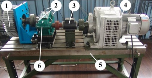
Fig. 9Gear after experiment
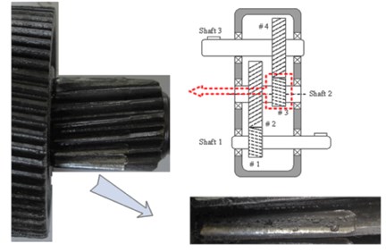
Fig. 10Special frequency band energy of vibration signal
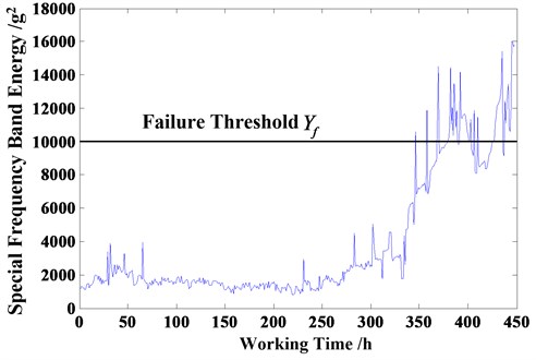
The total experimental time is 450 hours, the gear after experiment is shown in Fig. 9. As shown in Fig. 10, the special frequency band energy of vibration signal presents that degradation process of gearbox is obviously two-stage process. Using linear fitting analysis, degradation parameters of gearbox are obtained as follows: (12, 252), (76, 1302), [0, 450], 1. Meanwhile, the failure threshold is evaluated as = 10000g2.
Based on the proposed model and maintenance policies, optimal results for different maintenance policies of gearbox are shown in Table 4. Because the degradation rate of second stage for two-stage deteriorating mode system is faster than the first stage, the alarm threshold and inter-inspection time for the second stage should be smaller than the first stage. The initial inter-inspection time of time-depended maintenance policy is larger than the inter-inspection time of global maintenance policy , but inter-inspection time of time-depended maintenance policy is smaller and smaller with working time, as a result the expected cost make a decrease of 0.0108 from . The alarm thresholds of the first stage for adaptive and simplified adaptive maintenance policy , are both larger than alarm threshold of global maintenance policy , but the alarm thresholds of the second stage , are both smaller than . Meanwhile, the inter-inspection times , both between and . These phenomena conform to the conjecture in modeling. If use adaptive or simplified adaptive maintenance policy, the average long-run cost can reduce 9.29 %, 6.43 %, respectively. It can be seen that adaptive maintenance policy is the best method for gearbox.
Table 4Optimal results for different maintenance policies
Policy structure | Optimal parameters | Expected cost | Impact |
Global | , | ||
Time-depended | , , | 0.0108 (3.64 %) | |
Simplified Adaptive | , , | 0.0191 (6.43 %) | |
Adaptive | , , , | 0.0276 (9.29 %) |
6. Conclusions
This paper is meant to investigate degradation modeling and maintenance decision-making methods for two-stage deteriorating mode system, where the degradation rate is usually small in the first stage and large in the second stage. To this purpose, degradation level modeling and reliability modeling based on cumulative damage model are studied at first place, then four kinds of maintenance policies (global, time-depended, adaptive, simplified adaptive) are studied and evaluated through their average long-run cost rate. The four kinds of maintenance policies are differentiated from alarm threshold and inter-inspection time.
Moreover, influence analysis of different parameters for maintenance policy is studied and proves that: (a) It is necessary to consider degradation process undergoing a sudden change in maintenance policy, suitable maintenance policy can help to improve system efficiency. (b) It is obvious that the average long-run cost rate is impacted by change-point distribution, shock strength and shock frequency.
The case study of degradation data analysis for gearbox life-cycle experiment shows that degradation process of gearbox presents obviously two-stage feature. In addition, it is helpful to reduce the average maintenance cost by choosing appropriate maintenance policy.
References
-
Grall A., Dieulle L., Brenguer C., Roussignol M. Continuous-time preventive maintenance scheduling for a deteriorating system. IEEE Transactions on Reliability, Vol. 51, Issue 2, 2002, p. 141-150.
-
Wang H. Z. A survey of maintenance policies of deteriorating systems. Europian Journal of Operational Research, Vol. 139, Issue 3, 2002, p. 469-489.
-
Noortwijk J. M. V., Kallen M. J. Optimal periodic inspection of a deterioration process with sequential condition states. International Journal of Pressure Vessels and Piping, Vol. 83, Issue 4, 2006, p. 249-255.
-
Noortwijk J. M. V., Frangopol D. M. Two probabilistic life-cycle maintenance models for deteriorating civil infrastructures. Probabilistic Engineering Mechanics, Vol. 19, Issue 4, 2004, p. 345-359.
-
Mitra F., Antoine G., Laurence D. On the use of on-line detection for maintenance of gradually deteriorating systems. Reliability Engineering & System Safety, Vol. 93, Issue 12, 2008, p. 1814-1820.
-
Saassouh B., Dieulle L., Grall A. Online maintenance policy for a deterioration system with random change of mode. Reliability Engineering and System Safety, Vol. 92, Issue 12, 2007, p. 1677-1685.
-
Deloux E., Castanier B., Berenguer C. Maintenance policy for a non-stationary deteriorating system. Annual Reliability and Maintainability Symposium, Las Vegas, 2008.
-
Wang W. B. A two-stage prognosis model in condition based maintenance. European Journal of Operational Research, Vol. 182, Issue 3, 2007, p. 1177-1187.
-
Wang Z., Huang H. Z., Li Y., Xiao N. C. An approach to reliability assessment under degradation and shock process. IEEE Transactions on Reliability, Vol. 60, Issue 4, 2011, p. 852-863.
-
Liu Y., Huang H. Z. Optimal replacement policy for multi-state system under imperfect maintenance. IEEE Transactions on Reliability, Vol. 59, Issue 3, 2010, p. 483-495.
-
Liu Y., Huang H. Z. Optimal selective maintenance strategy for multi-state systems under imperfect maintenance. IEEE Transactions on Reliability, Vol. 59, Issue 2, 2010, p. 356-367.
-
Ponchet A., Fouladirad M., Grall A. Assessment of a maintenance model of a multi-deteriorating mode system. Reliability Engineering & System Safety, Vol. 95, Issue 11, 2010, p. 1244-1254.
-
Si X. S., Wang W. B., Hu C. H., Chen M. Y., Zhou D. H. A Wiener-process-based degradation model with a recursive filter algorithm for remaining useful life estimation. Mechanical Systems and Signal Processing, Vol. 35, Issues 1-2, 2013, p. 219-237.
-
Minh D. L., Cher M. T. Optimal maintenance strategy of deteriorating system under imperfect maintenance and inspection using mixed inspection scheduling. Reliability Engineering and System Safety, Vol. 113, 2013, p. 21-29.
-
Qian C. H., Nakamura S., Nakagawa T. Cumulative damage model with two kinds of shocks and its application to the backup policy. Journal of the Operations Research, Vol. 42, Issue 4, 1999, p. 501-511.
-
Song S. L., Coit D. W., Feng Q. M., Peng H. Reliability analysis for multi-component systems subject to multiple dependent competing failure process. IEEE Transactions on Reliability, Vol. 63, Issue 1, 2014, p. 331-345.
-
Wang X. L., Jiang P., Guo B., Cheng Z. J. Real-time reliability evaluation based on damaged measurement degradation data. Journal of Central South University, Vol. 19, Issue 11, 2012, p. 3162-3169.
-
Zhao Z., Wang F., Jia M., Wang S. Preventive maintenance policy based on process data. Chemometrics and Intelligent Laboratory Systems, Vol. 103, Issue 2, 2010, p. 137-143.
-
Grall A., Berenguer C., Dieulle L. A condition-based maintenance policy for stochastically deteriorating systems. Reliability Engineering & System Safety, Vol. 76, Issue 2, 2002, p. 167-180.
-
Grall A., Dieulle L., Berenguer C., Roussignol M. Asymptotic failure rate of a continuously monitored system. Reliability Engineering & System Safety, Vol. 91, Issue 2, 2006, p. 126-130.
-
Dagg R. A. Optimal Inspection and Maintenance for Stochastically Deteriorating Systems. Ph.D. Thesis, the City University, London, 1999.
-
Dieulle L., Berenguer C., Grall A., Roussignol M. Sequential condition-based maintenance scheduling for a deteriorating system. European Journal of Operational Research, Vol. 150, Issue 2, 2003, p. 451-461.
-
Sheldon M. R. Stochastic Processes for Insurance and Finance. Wiley Series in Probability and Statistics, Johon Wiley & Sons, New York, 1996, p. 639.
-
Mitra F., Grall A. Condition-based maintenance for a system subject to a non-homogeneous wear process with a wear rate transition. Reliability Engineering & System Safety, Vol. 96, Issue 6, 2011, p. 611-618.
About this article

