Abstract
The damping force of elastomer buffer in shock environment is the research object of this paper. The impact experiment and data simulation are used to understand the whole mechanical system. Equation with velocity and damping force is used for modeling according to the specific type of the elastomer buffer. The data of velocity and damping force is obtained by experimental data collection and pretreatment. Genetic algorithm is used to identify parameters according to the time invariant feature of traditional model. Through the results of parameter identification by genetic algorithm it seems that the parameters have the time-varying characteristics. Therefore, time-varying method is used for parameter identification. Limited memory method, which is obtained by the improvement of traditional least square method, is used for time-varying parameter identification. And the fitting accuracy of the identification results is better than that of genetic algorithm. The numerical results prove that the model is effective and parameters are time-varying.
1. Introduction
Elastomer is also called viscoelastic material, it is a kind of new functional material based on silicone polymer and consisted of a series of flame retardant, compression agent, plasticizer and colorant [1]. The elastomer has the characteristics of viscous liquid and elastic solid at the same time. And this kind of material has unique molecular helical structure, this structure makes it has good compressibility, shear stability, high elasticity and temperature performance stability. So it has a wide application in the field of aviation, aerospace, weapons, ships, transport and bridges etc. [2]. With the increasing applications of elastomer, buffers base on elastomer have also been widely used. Elastomer buffer has the characteristics of small volume, simple structure and low cost. Elastomer buffer now has been widely applied to railway traffic, vehicles, ships and other fields. Over the years, the analysis and exploration of the damping process of elastomer buffer has been a hot research. For different application fields of elastomer buffer, accurate modeling of damping process is very meaningful to the study of mechanical system and noise reduction [3-5].
When the types of elastomer buffer and experimental environment are different, the damping parameter identification models are different. Accurate experimental subjects and establishing a right identification model directly determine the feasibility of damping parameter identification. The experimental object in this paper is a vertical impact process. According to the experiment, velocity-damping identification model is established. In the simulation phase, the wavelet denoising is used to filtering the experimental data [6].
The parameters are time invariant in the traditional velocity-damping model. Firstly genetic algorithm is used for parameter identification. The results of genetic algorithm show that the values of parameter are different when the strain amplitude is different. Then the parameters of the model are set time-varying and identification method for time-varying parameters is used. The traditional least square method shows the characteristic of data saturation when it is used to identify time-varying parameters and the error is high. Limited Memory Method can solve the problem of data saturation and can get results with higher precision [7, 8].
2. Identification model
2.1. Mechanical model of elastomer
Elastomer is a kind of viscoelastic material. It has the mechanical properties of elastic materials and viscous materials at the same time [9].
The strain is generated immediately when stress is performed on elastic material. And elastic material itself has recovery ability. When the stress released, it can go back to the original state immediately. So the stress-strain curve of elastic material is linear as shown in Fig. 1(a).
When stress performed on viscous material, strain is generated gradually. Viscous material cannot recovery when stress is released. When the stress in positive direction reduces to 0, the strain in positive direction reaches to maximum. When the stress is increased in opposite direction, the strain will decrease in positive direction. If the stress is released, the strain will maintain the current state. Fig. 1(b) shows the stress-strain curve of viscous material.
The stress-strain curve of viscoelastic material is shown in Fig. 1(c). When stress is performed on viscoelastic material, strain will be produced. When is from 0 to the maximum value , the strain will not increase to the maximum value immediately due to the characteristic of viscous material. Before the strain reaches the maximum value, the stress has fallen. This is because the movement of molecular chain segment is effected by the internal friction, and the strain cannot keep pace with the change of stress. Therefore, the reverse route does not go through the original route. When stress dropped to 0, the strain is a non-zero value; when the stress continues to increase in the opposite direction, after reaching the maximum value , it will traffic back to the point by a new route to complete a cycle. It can be seen that the speed of strain is lower than the change speed of stress. It is called hysteresis phenomenon, which is dynamic viscoelasticity. The route of stress and strain forms a closed loop, which is called the hysteresis curve. When the stress is released, the strain will reduce to 0 gradually because it has the characteristic of elastic material.
Fig. 1Stress and strain curves of different materials
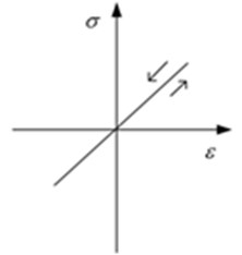
a) Elastic material
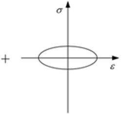
b) Viscous material
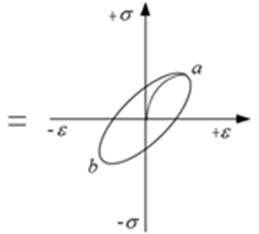
c) Viscoelastic material
2.2. Elastomer buffer
There are two kinds of elastomer buffer according to different motion styles, translational buffer and rotational buffer [10, 11]. Translational buffer is used in this paper and it has two types of structure, single rod buffer and double rod buffer. The experiment in this paper is performed in shock environment and one end of the buffer needs to be fixed. Therefore the translational buffer of single rod is chosen for the research.
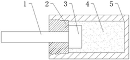
The structure of the elastomer buffer which is used in this paper is shown in Fig. 2. It is a single rod elastomer buffer. This kind of damper has a closed chamber, which is filled with viscoelastic fluid damping material. When elastomer is impacted by external load, the buffer piston rod is pressed into the cavity. The damping material flows through the annular gap formed by piston and cylinder wall. The damping medium in cavity is compressed and the internal pressure increases, and that caused the elastic force to the piston rod. At the same time, the piston head and damping structure produce great friction with the viscous damping medium. When the speed is higher, more viscous resistance will be produced. The impact kinetic energy can be turned into heat energy and elastic potential energy, which can be released in a very short time to achieve the effect of energy absorption. The elastomer also has good elasticity, which means, the volume will shrink under great external force. When the external pressure is up to 500 MPa, the compression ratio is not less than 17 % of the initial volume. When the external force is removed, the elastomers will automatic reset and release energy storage. And from Fig. 2, the numbers 1 to 5 represent piston rod, cylinder head, piston, resilient rubber and cylinder block.
Fig. 2Schematic diagram of elastomer buffer structure
2.3. Identification model
Energy buffer device can be manufactured according to different materials, energy dissipation mechanisms and structures. The experiment in this paper was performed in the shock environment. Speed-damping model is widely used for elastomer buffer in shock environment, which is shown as Eq. (1):
where is damping force, is damping coefficient, is the relative velocity between the piston and cylinder body and is velocity correlation coefficient (the larger its value, the smaller buffer’s nonlinear degree).
The model Eq. (1) shows is nonlinear. The complexity of nonlinear model is higher than that of linear model in the process of fitting. If it can be transformed into linear model, the fitting effect will be better. In order to linear fitting, logarithm was used on both sides of the formula which is shown as Eq. (2):
After the transformation above, the parameters need to be identified are linear parameters and . The data and can be obtained by the calculation of the damping force and velocity.
3. Identification algorithms
The elastomer material can be affected by the environment. The mechanical properties may be changed when temperature and strain amplitude are different. In the previous study, the parameters of identification model are fixed values. In this paper, the parameters are assumed as dynamic and identification method of dynamic is used. The model with fixed parameters will be identified by Genetic Algorithm. Model with dynamic parameters will be identified by Limited Memory Method.
3.1. Genetic algorithm (GA)
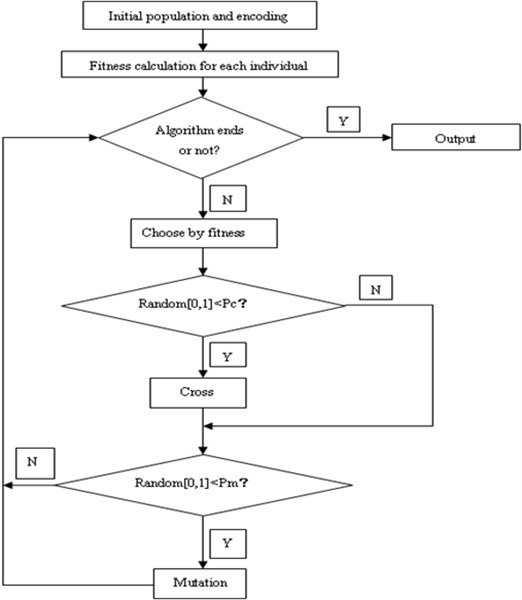
GA is an adaptive probabilistic optimization technique. It is based on genetic evolution mechanism [12, 13]. GA starts from a random initial population in latent solution space. After setting up initial population, individuals evolve according to the fitness standard which will gradually get better solution in each generation than before. In each generation, individuals can cross or mutate by certain probability to produce new ones. The optimal solution of the last generation can be used to solve the system problem.
There are many advantages of GA over traditional optimization algorithms: The search process does not need to consider whether the function is continuous; the algorithm is based on parallel calculation, which can decrease the calculation quantity and improve the efficiency; all calculations are only based on one fitness function, which is used to estimate individual’s fitness; the result from GA can be applied to solve problem directly and several optimal solutions can be given by GA.
The essence of GA involves the encoding of an optimization function as arrays of hits or character strings to represent the chromosomes, the manipulation operations of strings by genetic operators, and the selection according to their fitness in the aim to find a solution to the problem concerned. This is often done by the following procedure: encoding; defining a fitness function; creating a population; selecting an individual with high fitness; performing crossover and mutation to build a new population and continue to select individual until the optimal individual has been selected; and decoding the results to find the optimal solution to the problem. The process of GA is shown in Fig. 3.
Fig. 3Flow chart of GA
3.2. Limited Memory Method (LMM)
The least square method (LSM) is a relatively mature algorithm. It has been widely used in scientific experiments and engineering technology. With the development and popularization of modern computer, LSM shows more powerful vitality. LSM is used for solving the problem of how to find reliable value from a set of measurements. Its basic principle is: a group of data (, , 1, 2, …, ) are obtained, and try to find a best fitting curve in which the difference quadratic sum of the value of each point on the curve and measured value is minimum.
In the design of experiments, in order to reduce the error, multiple point measurement is performed. The number of the equations is far more than that of undetermined parameters. These equations are called inconsistent equation group. The equations transformed by LSM are called the normal equations (Here the number of equations is equal to the number of undetermined parameters). The undetermined parameters can be calculated by the normal equations.
The LSM is simple and practical, and its recursive algorithm is convergence and reliable. When the noise is white noise, the estimates can be unbiased, consistent and efficient. But with the growth of data, LSM will show the phenomenon of data saturation so that the recursive algorithm loses correction ability slowly. And the LSM cannot solve the problem of dynamic parameter identification. In that case, limited memory was introduced to LSM and the recursive algorithm called Limited Memory Method was obtained. LMM can solve the problem of data saturation caused by LSM.
LSM for estimating the time-varying parameters will produce great error, and can only track the trend of the time-varying parameters. This is because that when parameters change with time, new data will be submerged by old data if LSM is used. The characteristics of time-varying cannot be reflected. Therefore, the parameter identification method for time-varying system should pay special attention to the new data. LMM solves the problem of weak tracking according to a finite old data. When is equal to , the last observation value is . Then the recursive formula of the method is shown in Eq. (3), Eq. (4) and Eq. (5):
In order to keep the length of data window, the recursive formulas can be obtained in Eq. (6), Eq. (7) and Eq. (8):
3.3. A numerical example
Here is a simulation calculation example, which can show the advantage of LMM compare to LSM.
The linear time-varying model is given as follows:
where:
The true values of time-varying parameters are given by Eq. (11):
where is sampling period and equal to 0.001.
An input signal, which has a pseudo white noise sequence with signal noise ratio (SNR) 10:1, is given to the system of Eq. (9). The analytic output sequences are calculated out. And then special measurement noises are added to the analytic output sequences, which can be the actual output data. LSM and LMM were used respectively to perform parameter identification with the actual output data. The length of sample data is 2500 and the window length of LMM is 50.
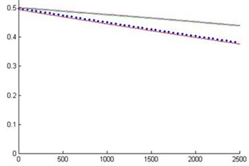
The numerical calculation result of system identification is shown in Fig. 4, which shows the identification result of parameter , , and by LSM and LMM. In the figures, the dotted line shows the true value of parameter, red line represents the identified parameters by LLM and the black line represents the identified parameters by LSM.
Fig. 4Identification results of parameter a1, a2, b1 and b2
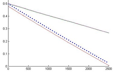
a) Identification of parameter
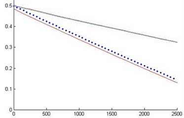
b) Identification of parameter
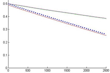
c) Identification of parameter
d) Identification of parameter
It can be seen from the results of numerical identification that when LSM is used for identification of time-varying parameters, the result in the beginning is close to the true value. But the error between result and true value will be larger when time goes on. This method can only get the change trend of parameters instead of the true values. The ability of LSM to track the time-varying parameters is far less than that of LMM. For the time-varying parameters, using LMM can obtain accurate identification results.
4. Study case
4.1. Experimental installation
According to the actual experimental environment and the characteristics of viscoelastic materials, the most common structure of single rod and ring type is chosen. The task book is given according to the laboratory equipment: the maximum impact velocity is 4 m/s, buffer stroke is 200-300 mm. The JRH-95V695 type elastomer buffer is chosen, and the capacity is 0.113 J. Dynamic viscosity elasticity is 2.0×10⁵ mPa⋅s, and the density is 0.95. The structure size is shown in Fig.5, and the internal structure parameters are shown in Table 1.
Fig. 5Structure diagram of elastomer buffer

Table 1Parameters of elastomer buffer
Parameters | Cylinder inner diameter | Piston rod diameter | Piston diameter | Piston thickness | Gap aperture |
Value (mm) | 75 | 30 | 50 | 25 | 15 |
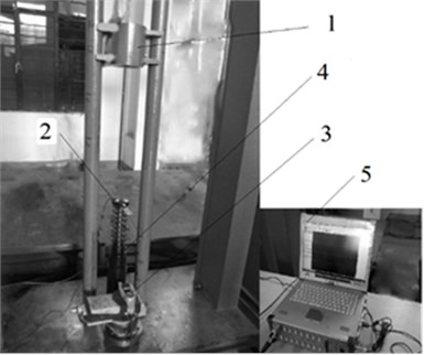
The measuring system for the experiment includes: signal receiver, laser displacement sensor and data acquisition system. Before the experiment, the buffer is fixed on the base. The impact hammer with quality of 30 kg was put in a suitable height. Then let the hammer fall free along the rail and impact the piston rod of buffer. The variation rule of displacement during the impact process was recorded by laser displacement sensor and data acquisition system. The actual installation of measuring equipment and elastomer buffer is shown in Fig. 6. And from Fig. 6, the numbers 1 to 5 represent impact hammer, signal receiver, laser displacement sensor, elastomer buffer and data acquisition equipment.
Fig. 6Schematic diagram of equipment
As the elastomer material can be affected by the strain amplitude, that is, when the strain amplitude is different, the parameters of buffer will change. Therefore, in order to verify this feature, two different sets of experiments are performed, in which different strain amplitude would be produce. Then the characteristics can be verified by parameter identification.
4.2. Data processing
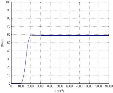
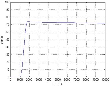
During the falling process, displacement information of the hammer was collected by laser displacement sensor with sampling frequency of 10 KHz. After the displacement information was collected, acceleration information could be obtained by two differential operation of displacement. Combined with the quality of the hammer, the damping force time curve could be obtained. During the falling process, there would be noise and vibration interference. Therefore, the data need to filter so that the accuracy of data can be ensured. By adjusting the initial height of the hammer, displacement-time curves of different initial velocity can be obtained. Thus the damping force time curves of different initial velocity can also be gained.
Two different initial heights, 300 mm and 700 mm were used to perform the low speed test and high speed test in this paper. The parameter identification for the two sets of data was used to verify the validity of the identification model. The displacement-time diagrams of low speed and high speed are shown in Fig. 7.
The acceleration-time diagrams of low speed and high speed are shown in Fig. 8.
Fig. 7Displacement-time diagrams
a) Low speed
b) High speed
Fig. 8Acceleration-time curves
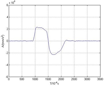
a) Low speed
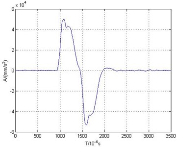
b) High speed
It can be seen from Fig. 8 that after piston rod impacts with the hammer, the motion of piston rod has two phases: acceleration phase and deceleration phase. In the acceleration phase, the elastomer material of the buffer has not yet started to flow when the piston rod begins to move. Therefore the damping forced in the acceleration phase is not generated by the flow of elastomer. In the deceleration phase, elastomer material starts to flow and generate damping force, so this paper extracts the velocity and damping force curve of the deceleration phase for research.
Through the calculation, the velocity and damping force curves during the deceleration phase are shown in Fig. 9.
Fig. 9Damping force curves
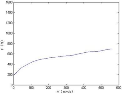
a) Low speed
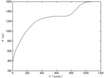
b) High speed
4.3. GA for parameter identification
According to Eq. (1), parameter identification is performed with GA respectively in low speed group and high speed group. In GA, the size of population 100; the iterations 100; crossover probability 0.8; mutation probability 0.05 and 10 bit binary code is chosen as the encoding mode. The algorithm is performed 100 times. The optimal parameters of each time are shown in Fig. 10. The result having the minimum fitting error is selected as the optimal solution. The fitting results are shown in Fig. 11 and Table 2.
Fig. 10Optimal parameters of GA for 100 times
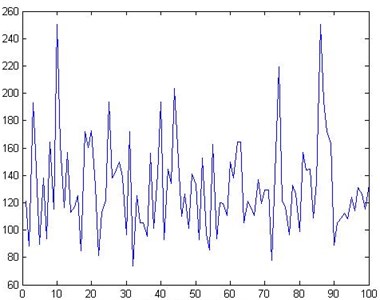
a) Parameter of low speed group
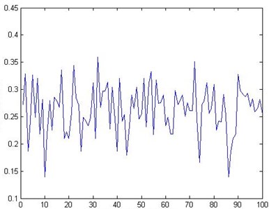
b) Parameter of low speed group
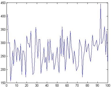
c) Parameter of high speed group
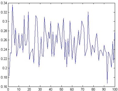
d) Parameter of high speed group
Fig. 11Fitting results by GA
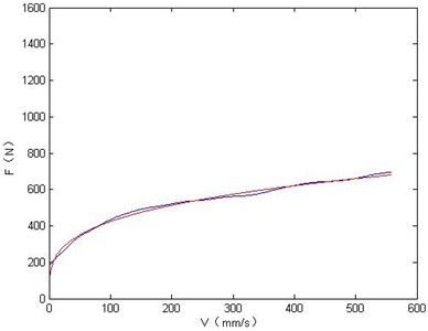
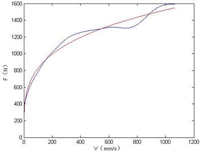
Table 2Identification result of GA
Speed type | Strain amplitude / mm | / N∙(m/s)-1 | Error | |
Low speed group | 58.62 | 169.74 | 0.2747 | 7.41×10⁴ |
High speed group | 72.22 | 224.37 | 0.2649 | 7.89×10⁵ |
4.4. LMM for parameter identification
According to the analysis of the results obtained from GA, when the strain amplitude is different, the results of time-invariant parameters will change. Therefore LMM is chosen for the time-varying parameter identification according to Eq. (2). The memory length is set by 50 and parameter identification is performed respectively in low speed group and high speed group. The fitting results are shown in Fig. 12.
Fig. 12Fitting results by LMM
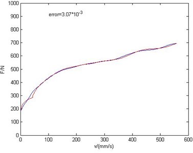
a) Low speed group
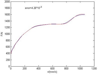
b) High speed group
The time from the elastomer buffer starting deceleration to it stopping motion is divided into 5 parts. Parameters of six moments from to are shown in Table 3 according to time sequence.
Table 3Identification results of LMM
Speed type | Parameter | ||||||
Low speed | 0.3895 | 0.3752 | 0.2781 | 0.2516 | 0.2784 | 0.2194 | |
Low speed | / N∙(m/s)-1 | 80.83 | 107.07 | 145.61 | 133.08 | 161.93 | 184.67 |
High speed | 0.3552 | 0.4270 | 0.3012 | 0.2425 | 0.2014 | 0.1625 | |
High speed | / N∙(m/s)-1 | 89.92 | 110.29 | 146.35 | 181.44 | 220.45 | 265.38 |
5. Conclusions
The elastomer material can be affected by the strain amplitude, when the strain amplitude is different, the parameters of the model will change. From the identification results of GA, it can be seen that when the strain amplitude is different, the results of parameter identification are not the same. With the increase of strain amplitude the damping coefficient increases and velocity correlation coefficient decreases. When time-invariant identification method is used, the fitting error will be larger as initial velocity increasing.
When LMM is used for parameter identification, the changing trend of parameter result is the same with results of GA, and LMM can effectively track the parameters and gets the parameter values with high accuracy.
The damping force model of elastomer buffer in shock environment is nonlinear. Through linearizing the nonlinear equation, the original parameters will be obtained by inverse logarithmic operation. This method can guarantee the accuracy of the premise and greatly improve the efficiency of the algorithm. The correctness of the model is confirmed by identifying the model parameters with GA and LMM.
References
-
Wong Dagen, Lu Zhuhun, Xu Bin Experimental study on mechanical properties of viscous damper. World Earthquake Engineering, Vol. 18, Issue 4, 2002, p. 30-34, (in Chinese).
-
Zhou Guangqiang, Yang Lina, Yang Aijun, Sun Zhongzhang Research progress on characteristics of elastomer buffer. Silicone Material, Vol. 25, Issue 1, 2011, p. 40-43, (in Chinese).
-
Wang Gancheng, Jiao Sujuan, Sun Jinya, Li Hongguang Shock experiments research and modeling analysis of elastomer damper. Noise and Vibration Control, Vol. 6, 2010, p. 55-62.
-
Park S. W. Analytical modeling of viscoelastic dampers for structural and vibration control. International Journal of Solids and Structures, Vol. 38, 2001, p. 8065-8092.
-
Gusella V., Terenzi G. Fluid viscous device modeling by fractional derivatives. Structural Engineering and Mechanics, Vol. 5, Issue 2, 1997, p. 177-191.
-
Shi Xianjun, Liao Jian, Ma Changli, Zhang Rong GLS parameter identification and simulation based on matlab. Computer and Digital Engineering, Vol. 37, Issue 8, 2009, p. 173-175, (in Chinese).
-
Li Wenyu, Du Hong, Liu Yanbin Application of least square method based on limited memory in parameter identification. Natural Sciences Journal of Habbin Normal University, Vol. 23, Issue 4, 2007, p. 23-25, (in Chinese).
-
Liu Cong, Sun Xiuxian, Li Haijun An identification method combing forget factor with limited memory method. Electronics Optics and Control, Vol. 13, Issue 1, 2006, p. 48-66, (in Chinese).
-
Jia J. H., Shen X. Y., Hua H. X. Viscoelastic behavior analysis and application of fractional derivative Maxwell model. Journal of Vibration and Control, Vol. 13, 2007, p. 385-401.
-
Lee D., Taylor D. P. Viscous damper development and future trends. The Structural Design of Tall Buildings, Vol. 10, 2001, p. 311-320.
-
Pekcan G., Mander J. B., Chert S. S. The seismic response of a 1:3 scale model R. C. structure with elastomericspring dampers. Earthquake Spectra, Vol. 1, Issue 2, 1995, p. 249-267.
-
Taboada A., Espiritu Jose F., Coit David W. MOMS-GA: a multi-objective multi-state genetic algorithm for system reliability optimization design problems. IEEE Transactions on Reliability, Vol. 57, Issue 1, 2008.
-
Ahn Youngjun, Park Jiseong, Lee Cheol-Gyun, Kim Jong-Wook, Jung Sang-Yong Novel memetic algorithm implemented with GA and MADS for optimal design of electromagnetic system. IEEE Transactions on Magnetics, Vol. 46, Issue 6, 2010.
About this article
This is supported by the National Major Instrument Project, 2013YQ4707650802.
