Abstract
Acoustical signals from mechanical systems reveal the operational status of mechanical components, which can be used for machinery condition monitoring and fault diagnosis. However, it is very difficult to extract or identify the acoustical source features as the measured acoustical signals are mixed signals of all the sources. Therefore, this paper studies on the source separation and identification of acoustical signals using principal component analysis and correlation analysis. The effectiveness of the presented method is validated through a numerical case study and an experimental study on a test bed with shell structures. This study can provide pure acoustical source information of mechanical systems, and benefit for machinery condition monitoring and fault diagnosis.
1. Introduction
The vibration and acoustical signals caused by the collisions and frictions of mechanical components provide important information of the operating conditions, and thus benefit for machinery condition monitoring and fault diagnosis. However, the measured vibration and acoustical signals normally are the mixed signals of all the source signals, and cannot be directly used for feature extraction due to the complicated waveforms. Therefore, it has great significance to separate the mixed signals into unrelated components, and recover the pure source information for machinery condition monitoring and fault diagnosis.
Generally, the measured acoustical signals are mixed signals of all the source signals with the transmission effects of mechanical structures. Therefore, they just can provide rough information of the mechanical systems. To reveal the mixing mechanism of acoustical signals, recently many researchers have devoted their efforts on the transmission characteristics of different mechanical structures. Vigran T. E. [1] described a simple method to account for the effect of point and line connections in double leaf constructions. Doutres O. [2] proposed a practical impedance tube method to optimize the sound transmission loss of double wall structure by concentrating on the sound package placed inside the structure. Dijckmans A. [3] presented a wave based model to predict the niche effect on sound transmission loss of single and double walls. Diaz Cereceda [4] presented a finite layer method for the computation of noise transmission through double walls. Sahu Kiran [5] studied on the active control of harmonic sound transmitted through soft cored sandwich panels into a rectangular enclosure. Shafer Benjamin [6] predicted the sound transmission loss through traditional wall and ceiling building partitions. Guillaume G. [7, 8] presented an original time domain approach applied to outdoor sound propagation under meteorological effects. All these studies researched on the transmission characteristics of different structures, and can benefit for a passive vibration and sound monitoring and control. However, sometimes it is a difficult and unnecessary task to build a precise model of the acoustical transmission for complex structures.
To clearly reveal the operating conditions of mechanical systems, signal processing methods are developed to extract the source features hidden in the noisy measured signals, and provide pure and clear source information for machinery condition monitoring and fault diagnosis. Principal component analysis (PCA) is a traditional and effective method to separate the linearly mixed signals into unrelated components, and has been applied to solve the source separation problems in many fields. Kramer M. A. [9] presented a nonlinear principal component analysis using auto-associative neural networks. Moore B. C. [10] investigated of PCA in linear systems controllability, observability, and model reduction. Tipping M. E. [11] proposed a probabilistic principal component analysis and gave illustrations. Zou H. [12] introduced sparse principal component analysis (SPCA) using the elastic net to produce modified principal components with sparse loadings. Candes E. J. [13] proposed a robust principal component analysis that can recover the principal components of a data matrix even though a positive fraction of its entries are arbitrarily corrupted. In engineering applications, PCA has attracted a worldwide attention and been widely applied to many fields, such as image fusion [14], flaw recognition [15], ECG feature extraction [16], data dimension reduction [17], and traffic identification [18]. On vibration and acoustical signal analysis, Antoni J. [19] addressed the issues of blind separation of vibration components. Cheng W. studied the source number estimation [20], source separation [21] and source contribution evaluation [22] methods for mechanical systems. In this paper, PCA is applied to acoustical source separation and identification, and the separation performances for typical acoustical signals are quantitatively evaluated through a numerical case study and an experimental study on a test bed with shell structures.
The remainder of this paper is organized as follows. In Section 2, basic theories and key algorithms of principal component analysis are introduced. In Section 3, the separation performance of principal component analysis is tested by a numerical case study. In Section 4, principal component analysis is applied to separate and identify acoustical signals of a test bed with shell structures. In Section 5, the conclusions of this study are summarized.
2. Theories of principal component analysis
2.1. Fundamental theories
The inner production of random vectors and is defined as the projection of random vector with zero-mean and dimensions on the unit vector with dimensions:
The projection vector is also a random vector, and it has zero mean and variance :
where is the covariance matrix of .
From Eq. (2), the variance of is a function of unit vector :
If the unit vector makes the variance function extreme, there will have:
where is a small disturbance of :
Combining Eq. (3) with Eq. (5), and ignoring the third part, there has:
From Eq. (4), can be replaced by :
From the theory, any disturbance of is not allowed. But in real calculation, small disturbance of is allowed in the condition that:
Considering Eq. (2), the disturbance vector must be:
Therefore, the disturbance vector must be orthogonal with the vector , which means the disturbance on the vertical direction is allowed.
To make vectors have the same scale, a scale factor is used. Thus there has:
The sufficient and necessary condition of Eq. (11) is:
From the basic theories, it can be concluded that the eigenvector of the covariance matrix for the random vector with zero-mean represents the principal direction, and the variance function has the extreme value in this principal direction. Furthermore, the scale factor or eigenvalue in this direction is the extreme value of variance function .
2.2. Principal component analysis
As the unit vector has possible solutions, the random vector will have possible projections. Specially, is the projection of on the unit vector :
The vector that satisfying Eq. (13) is defined as a principal component of the random vector . All the principal components can be expressed as:
The reconstructed vector thus can be denoted as:
2.3. Correlation analysis
For mechanical systems, some information of the sources normally can be known priori by the theory study or instructions. Therefore, correlation analysis can be used to evaluate the separation performances of PCA algorithm and identify the sources. For discrete signals and , the correlation coefficient is defined as:
where:
and is the data length.
3. Numerical case study
In this section, typical vibration and acoustical signals of mechanical systems are artificially generated to test the separation performance of the PCA algorithm. The source signals are: is a periodic wave of oscillating attenuation that simulates mechanical shocks; is a periodic wave that simulates frequency modulation; is a sinusoidal wave that simulates a vibration signal of rotational equipment; is a white noise that simulates noises produced by the environment and the structural transmission. The generating functions of sources are listed as follows:
where is a step function.
As the acoustical signals transmit from the sources to the measuring points through air, linear superposition is applied to artificially produce the mixed signals, and the mixing matrix is randomly generated as follow matrix:
The waveforms of the source signals and the mixed signals are shown in Fig. 1 and Fig. 2. Obviously, in Fig. 1 all the source signals have typical waveform features. However, it is very difficult to identify these features from the mixed signals in Fig. 2 as all the sources are coupling together. Therefore, PCA is applied to separate the mixed signals into principal components, and then these separated components are identified by the correlation analysis.
The waveforms of the principal components separated by PCA are shown in Fig. 3. Comparing Fig. 3 with Fig. 1, obviously the source signal is well separated. However, the other separated components still contain high frequency noises, which make these separated components are not clear and pure. To quantitatively evaluate the separating performances, correlation analysis are used. The correlation coefficients between all the sources and the principal components are shown in correlation coefficient matrix : the correlation coefficients between the separated components , , and and the source signals , , and are 0.97, 0.68, 0.78 and 0.90 respectively, which also indicates that the source signals and are well separated, while the other two source signals are not completely separated:
Fig. 1Waveforms of the source signals
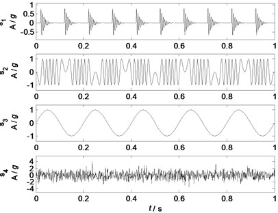
Fig. 2Waveforms of the mixed signals
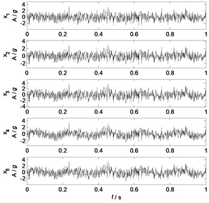
Fig. 3Principal components by PCA
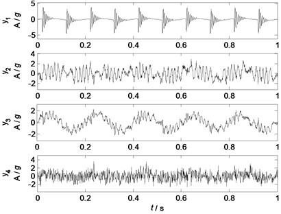
Fig. 4Principal components with low pass filtering
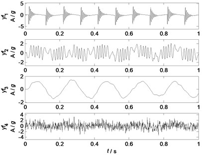
To enhance the separating performance of PCA and make the separated principal components more clearer and purer, the low-pass filtering is applied for separated signals and . The cut-off frequencies of separated components and are 110 Hz and 25 Hz respectively. Waveforms of the filtered principal components are shown in Fig. 4. Obviously, all the separated components are very similar to the related source signals. The correlation coefficients between all the sources and the filtered principal components are shown in correlation coefficient matrix : the correlation coefficients between the separated components , , and and the source signals , , and are 0.97, 0.92, 0.98 and 0.90 respectively, which indicates that all the waveform information of the source signals are well separated. Therefore, the PCA algorithm can separate the linearly mixed signals into uncorrelated components, which can extract rough source information. With the prior knowledge of the sources, the separated components can be refined by filtering, and more clearer and purer source information can be recovered from the mixed signals.
4. Experimental case study
4.1. Introductions of the test bed
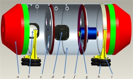
A test bed with shell structures is constructed to test the separation performance of PCA, which composes of four components: an end cover, a shell, two clapboards and supports. Rubber air springs are used to reduce the effects of the ground vibrations and environmental noises. Three acoustical sources are: two loudspeakers and one motor. The structures of the test bed is shown in Fig. 5.
Fig. 5The structures of the test bed: a) End cover; b) Loudspeaker I; c) Left clapboard; d) Loudspeaker II; e) Shell; f) Motor; g) Right clapboard; h) Rubber springs; i) Supports
Six sound pressure sensors are used to measure the acoustical signals, and they are located in six directions of the test bed with a distance of 500 millimeters. HBM Gen2i data acquisition system is applied to collect the acoustical data from these six sensors. The framework of the measuring system is shown in Fig. 6, and the testing parameters are shown in Table 1.
Fig. 6The framework of the measuring system
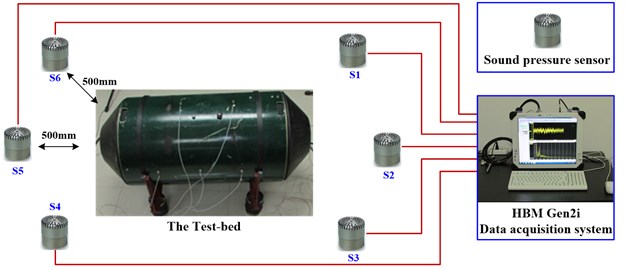
Table 1The testing parameters of the measuring system
Parameters | Values and units |
Sound pressure sensors | 6 |
HBM Gen2i data acquisition system | 1 |
Test bed with shell structures | 1 |
Sampling frequency | 10240 Hz |
Sampling length | 10 seconds |
Rotational speed of the motor | 2100 r/min (25 Hz) |
Frequency of loudspeaker I | 1500 Hz |
Frequencies of loudspeaker II | 2000 Hz (frequency modulation 50 Hz) |
4.2. Acoustical signals of the test bed
All the mixed signals are measured as all the sources are working together, and the acoustical signals from sensor 1, 3 and 5 are used as the mixed signals so as to satisfy the certainty solutions of PCA: the number of the mixed signals should be no less than the number of the source signals. Furthermore, the directions of these sensors represent a diversified mixing mode of all the sources.
Fig. 7Waveforms of the mixed signals
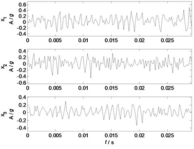
Fig. 8Spectrums of the mixed signals
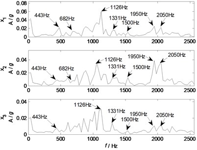
The waveforms and spectrums of the mixed signals are shown in Fig. 7 and Fig. 8 respectively. From waveforms in Fig. 7, it is difficult to identify the waveform features of the source signals except some periodic and sine waves, which indicate that the waveforms of the mixed signals are complicated, and normally signal processing method is required to extract the desired features. From spectrums in Fig. 8, some major components of 443, 682, 1126, 1331, 1500, 1950, and 2050 Hz are remarkable, which represent the characteristic features of the sources as the experimental settings combining with natural frequencies of the shell structure. Generally, the independent information of the source signals cannot be directly identified from the measured mixed signals as all the waveforms of source signals are coupling together.
4.3. Acoustical source separation
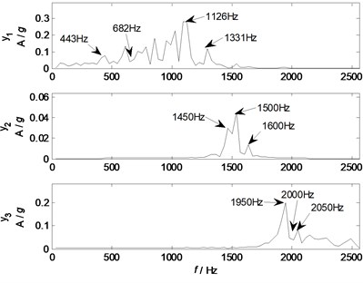
The PCA algorithm is applied to separate the mixed signals into unrelated components, and 3 independent components are extracted from the given mixed signals. To reduce the effects of noises, low pass filter is applied to remove the noisy components of the principal components and , the cut-off frequency of and are 1300 Hz and 1700 Hz, respectively. The waveforms and spectrums of the filtered principal components are shown in Fig. 9 and Fig. 10, respectively. Fig. 9 clearly shows that the waveform of the principal component has typically oscillating features, and the basic components are sine waves with different amplitudes, which are normally caused by the eccentric vibration of mechanical systems. The spectrums in Fig. 10 also show that the principal component has major components of 443, 682, 1126 and 1331 Hz. The waveform of the principal component has typical features of sine waves with amplitude modulation, and its spectrum also clearly shows the characteristic frequencies of 1450, 1500 and 1600 Hz. The waveform of the principal component has an obvious features of sine waves with amplitude modulation, and its spectrum contains three major components of 1950, 2000, and 2050 Hz.
Fig. 9Waveforms of principal components
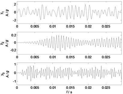
Fig. 10Spectrums of principal components
Comparing the spectrums of the principal components with the parameters of the experimental settings, it can be speculated that the principal component represents the typical feature of the source 1 from the motor, while the principal components and represent the typical features of the source 2 and 3 from the loudspeaker I and II, respectively. However, this is just based on the parameters of the experimental settings and it is still not convincing.
4.4. Acoustical source identification and validation
To intelligently identify the sources and validate the effectiveness of PCA in real mechanical systems, acoustical source signals are measured independently by the closest sensors in the condition that only one source is working with the given parameters. The independent source waveforms from sensor 1, 4 and 6 in the condition that only the motor, loudspeaker I, or loudspeaker II is working with the given experimental settings are shown in Fig. 11, and their spectrums are shown in Fig. 12.
Fig. 11Waveforms of the source signals
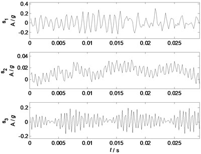
Fig. 12Spectrums of the source signals
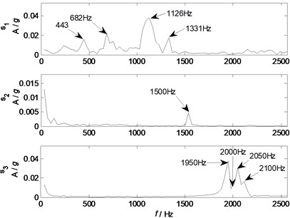
Comparing the waveforms and spectrums of the source signals with that of the filtered principal components, the waveforms of the filtered principal components are similar to that of the related source signals. However, due to the time delay and effects of the mixing mode and structural transmission, the waveforms of the principal components still cannot exactly recover the complete waveform information of the related source signals. Therefore, spectrum analysis is used to further validate the effectiveness of the principal components. Comparing Fig. 10 with Fig. 12, it is clear that the principal component recovers the major characteristic frequencies of 443, 682, 1126 and 1331 Hz contained in source signal 1; the principal component recovers the major characteristic frequency of 1500 Hz contained in source signal 2, and also has two other components of 1450 and 1600 Hz; the principal component recovers the major characteristic frequencies of 1950, 2000, 2050 Hz contained in source signal 3. Generally, all the major components of the source signals have been effectively separated by PCA with low pass filtering, and the major components of each sources can be traced by the spectrum analysis.
To quantitatively and intelligently identify the sources, the waveform correlation analysis is used to evaluate the similarity between the principal components and the sources. All the filtered principal components are made correlation analysis with all the sources, and the correlation coefficients are listed in the correlation coefficient matrix :
The correlation matrix shows that the correlation coefficients between the principal components and the related sources are 0.72, 0.64 and 0.74, which indicate relatively high correlation coefficients and high similarity between the principal components and the related sources (Liu [23] obtained waveform correlation coefficients of 0.77±0.03 for ECG signals with noises, and Farila [24] obtained correlation coefficients of 0.70±0.09 for non-stationary surface myoelectric signals); while the correlated coefficients between the principal components and the unrelated sources are less than 0.07, which indicates that all the principal components are unrelated to each other. Therefore, a threshold can be set as (in practice ) to intelligently identify and trace the acoustical sources, and the wide range of the threshold indicates that the acoustical sources can be well identified in real mechanical systems by PCA with low pass filtering.
After an effective source separation and tracing, the major features of the measured mixed signals can be extracted and traced, and then the related sources also can be traced and identified. With the source identification and tracing information, vibration and noise reduction, monitoring and control can be carried out. Furthermore, the pure source information from source separation can provide important features for machinery condition monitoring and fault diagnosis.
5. Conclusions
This paper presents the fundamental theory of principal component analysis, and validates the effectiveness of PCA for acoustical signals according to a numerical case study and an experimental study on a mechanical system with shell structures. The experimental study indicates that the acoustical sources can be effectively separated and intelligently identified.
In the numerical case study, four typical acoustical source signals of mechanical systems are effectively separated from five linearly mixed signals, and the correlation coefficients between the filtered principal components and the related source signals are all more than 0.90, which indicates a highly effective source separation for the given mixed signals. While in the experimental study on a mechanical system with shell structures, the correlation coefficients between the filtered principal components and the related source signals are all more than 0.64, which also reveals an effective acoustical source separation. If artificially giving a threshold for the correlation coefficients, all the acoustical sources can be intelligently identified and traced.
This work can provide pure source information for machinery condition monitoring and fault diagnosis, and the pure source information can also benefit for noise identification, reduction and control.
References
-
Vigran T. E. Sound transmission in multilayered structures – introducing finite structural connections in the transfer matrix method. Applied Acoustics, Vol. 71, Issue 1, 2010, p. 39-44.
-
Doutres O., Atalla N. Experimental estimation of the transmission loss contributions of a sound package placed in a double wall structure. Applied Acoustics, Vol. 72, Issue 6, 2011, p. 372-379.
-
Dijckmans A., Vermeir G. A wave based model to predict the niche effect on sound transmission loss of single and double walls. Acta Acustica United with Acustica, Vol. 98, Issue 1, 2012, p. 111-119.
-
Diaz Cereceda C., Poblet Puig J.,Rodriguez Ferran A. The finite layer method for modelling the sound transmission through double walls. Journal of Sound and Vibration, Vol. 331, Issue 22, 2012, p. 4884-4900.
-
Sahu K. C., Tuhkuri P. J. Active control of sound transmission through soft-cored sandwich panels using volume velocity cancellation. The Journal of the Acoustical Society of America, Vol. 134, Issue 5, 2013, p. 4190.
-
Shafer B. Determining sound transmission through damped partitions: challenges in theoretical prediction and laboratory testing. The Journal of the Acoustical Society of America, Vol. 134, Issue 5, 2013, p. 4003.
-
Aumond P., Guillaume G., Gauvreau B., Lac C., Masson V., Berengier M. Application of the transmission line matrix method for outdoor sound propagation modelling – part 2: experimental validation using meteorological data derived from the MESO-scale model MESO-NH. Applied Acoustics, Vol. 76, 2014, p. 107-112.
-
Guillaume G., Aumond P., Gauvreau B., Dutilleux G. Application of the transmission line matrix method for outdoor sound propagation modelling – part 1: model presentation and evaluation. Applied Acoustics, Vol. 76, 2014, p. 113-118.
-
Kramer M. A. Nonlinear principal component analysis using autoassociative neural networks. Aiche Journal, Vol. 37, Issue 2, 1991, p. 233-243.
-
Moore B. C. Principal component analysis in linear-systems – controllability, observability, and model reduction. IEEE Transactions on Automatic Control, Vol. 26, Issue 1, 1981, p. 17-32.
-
Tipping M. E., Bishop C. M. Probabilistic principal component analysis. Journal of the Royal Statistical Society Series B-Statistical Methodology, Vol. 61, 1999, p. 611-622.
-
Zou H., Hastie T., Tibshirani R. Sparse principal component analysis. Journal of Computational and Graphical Statistics, Vol. 15, Issue 2, 2006, p. 265-286.
-
Candes E. J., Li X. D., Ma Y., Wright J. Robust principal component analysis? Journal of the ACM, Vol. 58, Issue 3, 2011, p. 11.
-
Yi Z., Mayyas A., Omar M. A. Principal component analysis-based image fusion routine with application to automotive stamping split detection. Research in Nondestructive Evaluation, Vol. 22, Issue 2, 2011, p. 76-91.
-
Guo D.-D., Xia X.-J. Flaw recognition based on principal component analysis. Computer Engineering and Design, Vol. 33, Issue 5, 2012, p. 2031-2035.
-
Yun-Chi Y. An analysis of ECG for determining heartbeat case by using the principal component analysis and fuzzy logic. International Journal of Fuzzy Systems, Vol. 14, Issue 2, 2012, p. 233-241.
-
Rezghi M., Obulkasim A. Noise free principal component analysis: an efficient dimension reduction technique for high dimensional molecular data. Expert Systems with Applications, Vol. 41, Issue 17, 2014, p. 7797-7804.
-
Du M., Chen X. S., Tan J. An efficient method of P2P traffic identification based on wavelet packet decomposition and kernel principal component analysis. International Journal of Communication Systems, Vol. 27, Issue 10, 2014, p. 1476-1490.
-
Antoni J. Blind separation of vibration components: principles and demonstrations. Mechanical Systems and Signal Processing, Vol. 19, Issue 6, 2005, p. 1166-1180.
-
Cheng W., Lee S., Zhang Z. S., He Z. J. Independent component analysis based source number estimation and its comparison for mechanical systems. Journal of Sound and Vibration, Vol. 331, Issue 23, 2012, p. 5153-5167.
-
Cheng W., He Z. J., Zhang Z. S. A comprehensive study of vibration signals for a thin shell structure using enhanced independent component analysis and experimental validation. Journal of Vibration and Acoustics – Transactions of the ASME, Vol. 136, Issue 4, 2014, p. 041011.
-
Cheng W., Zhang Z. S., Lee S., He Z. J. Source contribution evaluation of mechanical vibration signals via enhanced independent component analysis. Journal of Manufacturing Science and Engineering – Transactions of the ASME, Vol. 134, Issue 2, 2012, p. 021014.
-
Liu H. T., Chang C. Q., Luk K. D. K., Hu Y. Comparison of blind source separation methods in fast somatosensory-evoked potential detection. Journal of Clinical Neurophysiology, Vol. 28, Issue 2, 2011, p. 170-177.
-
Farina D., Fevotte C., Doncarli C., Merletti R. Blind separation of linear instantaneous mixtures of nonstationary surface myoelectric signals. IEEE Transactions on Biomedical Engineering, Vol. 51, Issue 9, 2004, p. 1555-1567.
About this article

This work was supported by the projects of National Nature Science Foundation of China (No. 51305329), the China Postdoctoral Science Foundation (No. 2013M532032, No. 2014T70911), the Doctoral Foundation of Education Ministry of China (No. 20130201120040), and Basic Research Project of Natural Science in Shaanxi Province (No. 2015JQ5183).
