Abstract
Magnetic pulse forming (MPF) is a plastic deformation method that uses a high intensity magnetic field. Compared to the traditional forming process, this method is simple, and produces better surface quality of the molded product after processing. In this study, we maximized the MPF depth of a molded product using the results of an optimization study. In addition, we determined an optimal coil shape, the electrical energy in the capacitance, and the input voltage to the system. MAXWELL, commercial software, was used to calculate the forming pressure and its distribution induced by the electromagnetic field. MAXWELL was also used to determine the coefficients of approximation equations modeled from the pressure distribution, using the least squares method. Furthermore, the commercial structural analysis software ANSYS, and the commercial statistical analysis software PIAnO, were coupled for an analysis of the optimized design factor to find the maximum forming depth.
1. Introduction
Magnetic pulse forming (MPF) is a forming technique for the plastic deformation of a plate with a rate of 15 to 300 m/s using a high intensity magnetic field. If current is momentarily discharged to a forming coil, a Lorentz force is generated. The force acts on the work piece to generate the desired shape of the product [1].
MPF has been developed to compensate for the disadvantages of conventional forming processes such as stamping and hydroforming. The conventional processes require a long process time and a large facility. However, MPF needs only a small space, and offers fast processing speed because MPF use an electromagnetic force induced by a small coil [2, 3].
Lee et al. reported the design parameters of magnetic pulse forming [4]. They selected three design variables that have the greatest impact on forming depth: the number of turns of the forming coil, the capacitor’s stored electric energy, and the voltage applied during the forming process. Then, they analyzed how the variables affected the forming depth. They tried to maximize the forming depth by controlling the voltage, and suggested that if the assigned number of coil turns and capacitance are constant in the MPF system, then the voltage is proportional to the penetration depth [5].
Noh et al. investigated the displacement at several positions on the forming plate using a constant turn coil [6]. They performed five experiments with constant electrical energy and a constant number of coil turns, and measured the penetration depth [7]. To the best of our knowledge, no optimization study to date has considered the effect of the number of coil turns on the maximum penetration depth of an MPF system.
In our analysis of the effects of design parameters, the commercial software programs MAXWELL, ANSYS, and PIAnO were used. The electromagnetic software MAXWELL (ver16) was used to analyze forming pressure and its distribution. Using the forming pressure distribution results, the coefficients of the approximation equations were determined by using the least squares method. Using the approximation equation, the forming depth was calculated by using ANSYS structural analysis software (ver14.5). PIAnO statistical software (ver3.5) was used for the optimization of the forming depth.
2. Magnetic pulse forming
2.1. Structure and operating principle of a magnetic pulse forming device
The magnetic pulse forming equipment consists of forming and circuit parts, as shown in Fig. 1(a). The forming parts are comprised of a forming coil, plate, and die. Fig. 1(b) shows the cross section of the magnetic pulse forming device with fixed dimensions for the die and forming coil. As shown in this figure, the forming plate is located between the coil and forming die. As depicted in Fig. 1(c), the circuit is comprised of a capacitor, resistor, inductor, and charge/discharge switch. The charge/discharge switch turns the forming force on and off.
Fig. 1Schematic of magnetic pulse shaping device
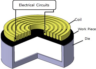
a) Magnetic pulse-forming system structure
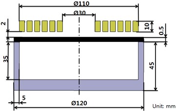
b) Cross section of the magnetic pulse forming device
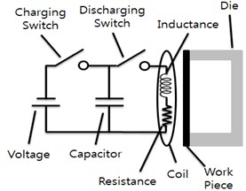
c) Electrical circuits
The principles of the magnetic pulse-forming device are depicted in Fig. 2. Fig. 2(a) shows the initial state. At this stage, the charging switch and discharging switch are in the OFF state. In the second stage as shown in Fig. 2(b), the charging switch is ON and the discharging switch is OFF. In the third step, shown in Fig. 2(c), the charging switch is OFF and the discharging switch is ON. When the electric energy in the capacitor is stored in a short time, the current starts to flow in the forming coil. At this time, induced electromotive force, as described by Faraday’s law, is exerted on the sheet. The force is equal to the rate of change of the magnetic flux passing through the closed circuit. The direction of the force is opposite to that of the current passing through the forming coil, as described by Eq. (1). The Lorentz force generated by the induced current and the magnetic field of the forming coil is forming pressure [8]:
where – electromotive force, – flux, – time.
Fig. 2Principle of magnetic pulse forming device
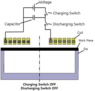
a) Initial state before forming
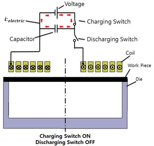
b) Charging capacitor
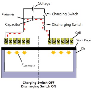
c) Capacitor discharge
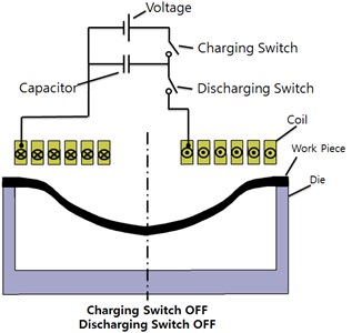
d) After forming
In the fourth stage, both the charging and discharging switch are in the OFF state. The plate formed by Lorentz force is shown in Fig. 2(d). The electrical energy has been discharged in the capacitor. In other words, the circuit turns back to the initial state. The Lorentz force is expressed as follows [9]:
where – current flowing through the conductor, – the length of the conductor, – the density of the magnetic flux, – the Lorentz force.
The Lorentz force acts in the vertical direction, which is toward the die face. In other words, the force direction is orthogonal to the magnetic field of the forming coil and the induced current.
2.2. Electromagnetic analysis of the initial model
In order to interpret the forming pressure and pressure distribution of the initial model, the commercial electromagnetic analysis program MAXWELL was used. 2-D cylindrical coordinates were used in the model as shown in Fig. 3. 2-D modeling was used instead of 3-D because 2-D analysis is more accurate.
Table 1Electrical property of copper, aluminum, and stainless steel
Copper | Aluminum | Stainless steel | |
Bulk conductivity | 530×106 | 330×106 | 11×106 |
Relative permittivity | 1 | 1 | 1 |
Relative permeability | 0.999 | 1.001 | 1 |
The materials used for the forming coil, plate, and die are copper, aluminum, and stainless steel, respectively. The electrical properties of these materials are given in Table 1.
The analysis contains the transient electromagnetic behavior. The total analysis time is 1 ms, and the time step was set to 5 μs. The “Auto Mesh” feature in the MAXWELL program was used to define the mesh size depending on the magnetic field density. Therefore, the mesh size is quite small in the dense field area. The forming voltage applied to the coil, the number of coil turns, and the coil resistance is shown in Table 2.
Fig. 4 shows the magnetic flux lines generated near the coil and forming plate. A higher magnetic density produces a higher forming force.
Table 2Voltage, the number of turns of the forming coil, and the resistance of the forming coil
Value | |
Input voltage (kV) | 15 |
Number of turns | 6 |
Resistance of coil (Ω) | 0.01 |
Fig. 3MAXWELL initial analysis model
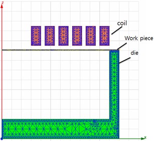
Fig. 4Magnetic flux lines
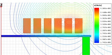
Fig. 5Current decreasing with time
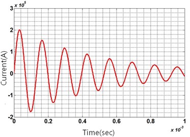
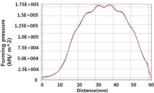
Our main interest is to characterize the displacement that determines the forming quality. Therefore, the forming pressure and forming pressure distribution should be considered since the two factors are the most related factors with respect to the displacement of the plate. As shown in Fig. 5, alternating current (AC) given to investigate the effects of the two factors. This time-varying voltage produces the corresponding forming pressure on the plate. As shown in Fig. 6, 200 steps produce a different forming pressure distribution. Among the 200 steps, the data generated at 5×10-005 produces the maximum forming pressure, and this was selected for the structure analysis described in next step. Fig. 7 shows the maximum value of forming pressure during the forming process simulation, which will be formulated to the numerical equation in Section 2.3.
Fig. 6Forming pressure distribution results from MAXWELL
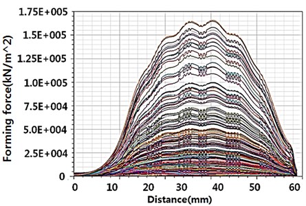
Fig. 7Maximum forming pressure
2.3. Numerical analysis of the initial model
The maximum forming pressure distribution, based on results from MAXWELL, was formulated for coupling with ANSYS. A formula describing the forming pressure distribution was generated using the fitting tool in MATLAB (ver2010b).
The maximum forming pressure can be decomposed from several harmonic functions, as shown in Eq. (3). A sinusoidal function of the 8th order was selected to model the maximum forming pressure distribution:
The least squares method was used in Eq. (5) to obtain the coefficients of the equation. is the square value of the residual value;, , denote the respective coefficient values; is the position of the plate, and is the residual. , , are defined at the minimum of the value. square, which is a measure of the reliability of the formula, is 0.9992. As previously mentioned, the graph shown in Fig. 6 was converted to a numerical equation using Eqs. (3) and (5). Table 3 shows fitting coefficients.
Table 3Fitting coefficients for Eq. (5)
1 | 3.321e+005 | 0.02515 | 0.06624 |
2 | 2.119e+005 | 0.04893 | 1.775 |
3 | 1.348e+005 | 0.1018 | –1.369 |
4 | 2.282e+004 | 0.257 | –1.374 |
5 | 1.547e+004 | 0.2281 | –2.863 |
6 | 5731 | 0.3628 | –1.609 |
7 | 8782 | 0.1048 | 2.338 |
8 | 2541 | 0.5743 | 1.227 |
2.4. Structural analysis of the initial model
ANSYS was used to analyze how the forming pressure affects the displacement of the plate. The previous formulation was used as the input to the ANSYS program. The main difference between the MAXWELL model and the ANSYS model is the forming coil that generates the electromagnetic field, because MAXWELL performs electromagnetic analysis and ANSYS performs structural analysis. Therefore, the forming coil was removed in the structural analysis using ANSYS.
The “Fixed Support” function in ANSYS was used instead of modeling the die in order to reduce computational cost. The properties of the plate and die are summarized in Table 4. The material used in the ANSYS analysis is aluminum alloy nonlinear (NL) and stainless steel NL. The stress and strain curve of each material is required for the analysis of plastic deformation in ANSYS. For example, the stress-strain curve shown in Fig. 8 was used to represent aluminum alloy NL.
Table 4Aluminum properties
Material | Density | Poisson‘s ratio | Yield strength |
Aluminum alloy NL | 2770 kg/m3 | 0.33 | 280 MPa |
Fig. 8Aluminum alloy NL stress-strain curve
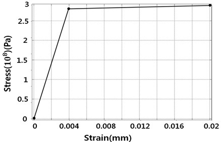
Fig. 9(a) shows the initial model for the structural analysis. In this figure, the fixed support indicates the area where the die and the plate meet. Cylindrical coordinates were used because the magnetic field follows the coil shape and the coil is cylindrical in shape. FE mode is created by auto mesh tool of MAXWELL. The number of elements is 625 using 2D cylindrical coordinate system.
The deformation and stress distribution are shown in Figs. 9(b) and (c). The center of the plate exhibits the maximum deformation. This result is related to the fixed support, where there is no displacement change. In other words, when pressure is exerted on the plate, both ends of the plate are fixed and the center of the plate is unconstrained as a result, the overall shape of the deformed plate is conical. The maximum deformation and maximum stress are 87.288 mm and 16.068 GPa.
Fig. 9ANSYS analysis
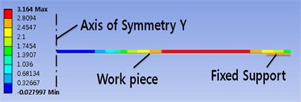
a) Initial state
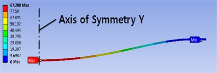
b) Total deformation
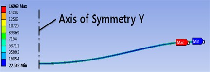
c) Von Misses stresses
3. Design problem definition
3.1. Design requirements
Our final goal is to maximize the forming depth. In this study we defined the variables that cause a change in depth as optimized parameters. The forming depth depends on the forming pressure and forming pressure distribution. These two factors mainly result from capacitance, input voltage, and the number of turning coils [11].
In an MPF device, the electrical energy is linearly proportional to the forming pressure. Due to this linear relationship, optimization is difficult. Hence, in this study, the optimized design values for capacitance, input voltage, and the number of coil turns are defined under a constraint of constant electrical energy.
3.2. Design parameters
For the design of the forming coil, three factors (width (), space (), and height ()) are defined as shown in Fig. 10. The simulation is divided into five cases as summarized in Table 6. Note that the area of the cross section is the same in all cases. This is because the volume of the coil is constant.
Table 6Number and dimensions of the forming coil turns
Turn | (mm) | (mm) | (mm) |
4 | 7.5 | 3.34 | 10 |
5 | 6 | 2.5 | |
6 | 5 | 2 | |
7 | 4.28 | 1.66 | |
8 | 3.75 | 1.43 |
The electrical energy () is a key factor affecting the forming pressure. The capacitor size () and input voltage () define the electrical energy (), as shown in Eq. (9). The initial value, lower limit, and upper limit for the design variables of the electrical energy are summarized in Table 7.
where – electric energy, – voltage, – capacitor.
Fig. 10Shape of the forming coil
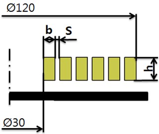
Table 7Design variables, initial value, upper limit, and lower limit
Design variables | Lower | Initial | Upper | Unit |
: number of coils | 4 | 6 | 8 | turns |
: capacitor | 200 | 281 | 500 | uF |
: voltage | 15 | 20 | 25 | kV |
3.3. Design problem formulation
The optimization of the problem, including the prescribed constraints, can be defined as follows (Eq. (10)):
where is the forming depth.
4. Optimization of the magnetic pulse forming device
The commercial software PIDO (ver3.5) was used to optimize Eq. (10). PIAnO, which provides the design of experiment (DOE), approximation, and optimization functions, was used in subsequent steps as shown in Fig. 11.
4.1. Design of experiments
DOE was performed to increase the accuracy of the designed model. The computational experiments were conducted by following the orthogonal array as shown in Table 8.
Fig. 11Design optimization procedure
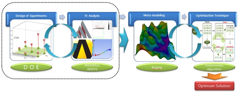
Table 8Experimental schedule
Case | Number of turns | Voltage (kV) | Capacitance (uF) | Displacement (mm) |
1 | 4 | 15 | 2 | 3.3045 |
2 | 4 | 15 | 3.5 | 14.488 |
3 | 4 | 15 | 5 | 44.113 |
4 | 4 | 20 | 5 | 23.223 |
5 | 4 | 20 | 2 | 64.529 |
6 | 4 | 20 | 3.5 | 41.269 |
7 | 4 | 25 | 3.5 | 78.485 |
8 | 4 | 25 | 5 | 122.6 |
9 | 4 | 25 | 2 | 22.636 |
10 | 6 | 20 | 3.5 | 95.208 |
11 | 6 | 20 | 5 | 148.74 |
12 | 6 | 20 | 2 | 33.41 |
13 | 6 | 25 | 2 | 102.12 |
14 | 6 | 25 | 3.5 | 180.99 |
15 | 6 | 25 | 5 | 53.546 |
16 | 6 | 15 | 5 | 52.195 |
17 | 6 | 15 | 2 | 18.805 |
18 | 6 | 15 | 3.5 | 95.093 |
19 | 8 | 25 | 5 | 511.47 |
20 | 8 | 25 | 2 | 184.11 |
21 | 8 | 25 | 3.5 | 269.01 |
22 | 8 | 15 | 3.5 | 60.418 |
23 | 8 | 15 | 5 | 94.401 |
24 | 8 | 15 | 2 | 33.987 |
25 | 8 | 20 | 2 | 96.861 |
26 | 8 | 20 | 3.5 | 172.14 |
27 | 8 | 20 | 5 | 327.32 |
4.2. Approximation techniques
A meta-model, called a Kriging model, was generated from the prescribed DOE. This statistical model is used to estimate an unknown value of interest through a linear combination of the known values [12]. In PIAnO, the estimated predicted square was 0.82, which is a reasonable value for our optimization problem.
4.3. Optimization
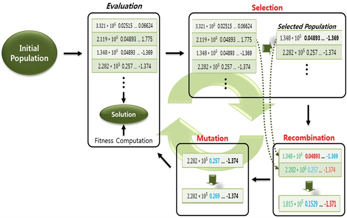
An evolution algorithm (EA) was used for the optimization procedure. This algorithm is based on a mechanism of real evolution in nature. The EA is a popular method for solving optimization problems. The algorithm generates a first population from the defined variables. It evaluates the fitness of individuals among the population and then selects the best parents, which represent the best optimized parameters. Based on the parameters, the parents mutate to find individual results having better fitness. This process is repeated to find the optimized solution, as shown in Fig. 12 [13, 14].
Fig. 12Full implementation process of an evolutionary algorithm
Population sizes are the number of the times that are analyzed in a generation and maximum number of generations is repetition number of generation. In addition, the total number of analysis is the product of the population size and the maximum number of generations and no of consecutive generations without improvement is the allowed number of unchanging repetitions generation, as shown in Table 9.
Table 9Parameters of the evolutionary algorithm
Parameter | Variable |
Population size | 100 |
Maximum number of generations | 250 |
Violated constraint limit | 0.003 |
No. of consecutive generations without improvement | 20 |
Mutation probability | 0.01 |
Selection probability | 0.15 |
4.4. Optimal design results
In our results for the optimal design using the meta-model (Opt_meta), the forming depth increased by 74.7 % compared to the initial model. However, the optimal design results can be changed based on the meta-model instead of the actual analytical model used in this research. The accuracy of the optimization results should be verified by analysis using MAXWELL and ANSYS software. To do this, the results of the Kriging model (Opt_meta) and the results of the actual analysis (Opt_real) were compared, as shown in Fig. 13. The Kriging model results (Opt_meta) and the ANSYS model results (Opt_real) were similar; therefore, we confirmed the high accuracy of the Kriging model’s prediction. The initial and optimal values of the design variables were compared, as shown in Table 10.
Fig. 13Performance index change
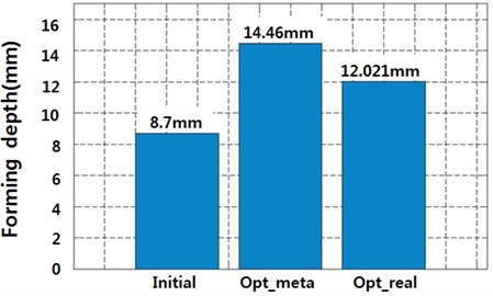
Table 10Values determined from the optimization results
Design variables | Lower | Initial | Optimal | Upper | Unit |
: number of coil turns | 4 | 6 | 8 | 8 | turns |
: capacitance | 200 | 281 | 356.8 | 500 | uF |
: voltage | 15 | 20 | 18.0148 | 25 | kV |
Fig. 14Forming pressure according to winding coil turns
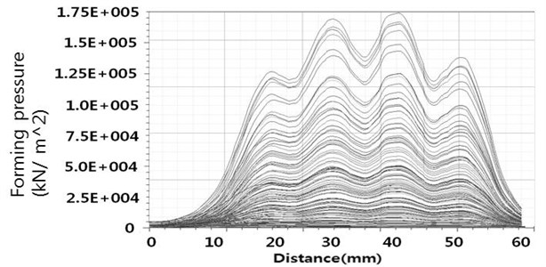
a) 4 turns
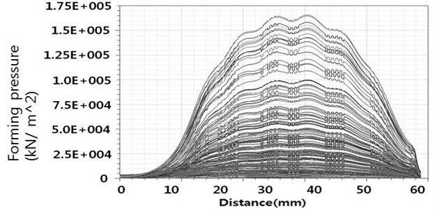
b) 8 turns
Fig. 14 shows how the forming pressure and forming pressure distribution affect the displacement of the plate. The case (Fig. 14(a)) with no uniform forming pressure distribution and high forming pressure has less penetration than the reverse case (Fig. 14(b)). In other words, a uniform pressure distribution with the low forming pressure case is better for deeper penetration. In this case, the number of coil turns was 8.
5. Conclusions
An optimization study was performed to increase the performance of a magnetic pulse forming device. The MAXWELL and ANSYS commercial software packages were coupled for the optimization process.
Fitting formula of the forming pressure was developed. The forming pressure and pressure distribution were obtained using the least squares method. Then, the result was formulated using an 8th-order harmonic function that was input to ANSYS. ANSYS was used to calculate the displacement of the plate.
Optimization was conducted by defining the variables and constraints. A computational DOE was performed using the orthogonal array (318). From the results, the meta-model was defined and the fitness was reviewed using the predicted -square value. An evolution algorithm was combined with the meta-model to find the optimized values of each design variable.
As a result, under constant electrical energy, the penetration depth can be increased from 87.288 to 138.48 mm. In summary, the number of coil turns has a great effect on the forming pressure distribution. Moreover, the electrical energy, which is controlled by a capacitor and the input voltage, affects the maximum forming pressure.
Regarding how the forming pressure and forming pressure distribution affect the displacement of the plate, the case with no uniform forming pressure distribution and high forming pressure has less penetration than the reverse case. If the electrical energy is not constant, the capacitor and input voltage should be assigned to the upper limit. However, the electrical energy was fixed because we wanted to simulate the case that has the same energy as that of the initial model. The capacitance was increased from 281 to 356.8 uF. The input voltage was reduced from 20 to 18 kV. Moreover, when the number of coil turns is increased, the pressure distribution becomes uniform, the capacitor size should be increased, and the input voltage should be decreased for maximum penetration.
We suggest that the results of this study can be used to guide the optimization of a process parameter combination to achieve the best performance for a magnetic pulse-forming device.
References
-
Rohatgi Aashish, et al. Electro-hydraulic forming of sheet metals: free-forming vs. conical-die forming. Journal of Materials Processing Technology, Vol. 212, Issue 5, 2012, p. 1070-1079.
-
Kang Beom-Soo, Bo-Mi Son, Jeong Kim A comparative study of stamping and hydroforming processes for an automobile fuel tank using FEM. International Journal of Machine Tools and Manufacture, Vol. 44, Issue 1, 2004, p. 87-94.
-
Zhang Shi-Hong Developments in hydroforming. Journal of Materials Processing Technology, Vol. 91, Issue 1, 1999, p. 236-244.
-
Lee Man Gi, Yi Hwa Cho, Shin Ki-Yeol, Kim Jin Ho Study on design parameters of magnetic pulse forming device. Journal of the Korean Society of Manufacturing Process Engineers, Vol. 10, Issue 2, 2014, p. 28.
-
Lee H. M., Kang B. S., Kim J. Development of sheet metal forming apparatus using electromagnetic lorentz force. Transactions of Materials Processing, Vol. 19, Issue 1, 2010.
-
Noh Hak Gon, Song Woo Jin, Kang Beom Soo, Kim Jeong Optimum coil design for electromagnetic forming by finite element method. Korean Society of Mechanical Engineers, Vol. 13, Issue 19, 2013, p. 240-241.
-
Noh Hak Gon, Park Hyeong Gyu, Song Woo Jin, Kang Beom Soo, Kim Jeong Effect of process parameters in electromagnetic forming apparatus on forming load by FEM. Journal of the Korean Society for Precision Engineering, Vol. 30, Issue 7, p. 733-740.
-
Krige D. G. A statistical approach to some basic mine valuation problems on the wit water stand. Journal of the Chemical, Metallurgical and Mining Society of South Africa, Vol. 52, Issue 6, 1951, p. 119-319.
-
Harvey George W. Harvey Etal. U.S. Patent No. 2.976.907, 1961.
-
Bernatt Joseph Fuse housing end caps secured by magnetic pulse forming. U.S. Patent No. 4.063.208, 1977.
-
Grinvald Amiram, Izchak Z. Steinberg On the analysis of fluorescence decay kinetics by the method of least-squares. Analytical Biochemistry, Vol. 59, Issue 2, 1974, p. 583-598.
-
Back T. Evolutionary Algorithms in Theory and Practice: Evolutionary Programming, Genetic Algorithm. Oxford University Press, Oxford, 1996.
-
Joeng M. J., Dennis B. H., Yoshimura S. Multidimensional clustering interpretation and its application to optimization of coolant passage of a turbine blade. ASME, Vol. 127, 2005, p. 215-221.
-
Fonseca Carlos M., Peter J. Fleming An overview of evolutionary algorithms in multi objective optimization. Evolutionary Computation, Vol. 3, Issue 1, 1995, p. 1-16.
About this article

This research was supported by Yeungnam University research Grant in 2015.
