Abstract
The nonlinear electromagnetic force can change the critical velocity of the projectile for a railgun. It corresponds to the resonance state in railgun. Here, the nonlinear electromechanical coupled dynamics equations for the railgun are proposed. Based on it, the equation of the nonlinear critical velocity of the projectile is given and the effects of the electromagnetic nonlinearity on the critical velocity of the projectile are investigated. Besides it, the effects of the fire velocity on the nonlinear critical velocity are studied as well. Results show that the critical velocity of the railgun system increases when the electromagnetic nonlinearity is considered, and the nonlinear critical velocity is influenced by the system parameters such as rail current, rail thickness, rail distance, etc. A FEM analysis package, ANSYS, is used to simulate dynamics performance of the railgun system and illustrate the analytical results about critical velocities of the railgun system. The results can be used to design dynamics performance of the railgun system.
1. Introduction
The railgun was proposed about one hundred years ago. It is an attractive electromagnetic gun due to its apparent simple design and the muzzle velocities up to 2.5 km/s for masses of several hundred grams have been demonstrated experimentally [1-3].
In the railgun, the vibration of the rail under the transient magnetic load may cause disturbances of the projectile trajectory. Therefore, the dynamic performance of the rail is of great importance for the railgun system. The first dynamic model of the electromagnetic railgun is one-dimensional beam model on an elastic foundation [4]. Then, the mechanical response of the railgun to the moving magnetic load was studied [5, 6]. For improving calculating accuracy, the axis-symmetric shell and two-dimensional solid models were used to study the resonance at critical velocities of the projectile [7]. The transient elastic waves in the railgun and their influence on armature contact pressure were analyzed [8, 9]. A 2D finite element model resting upon discrete elastic supports was used to analyze the transient performance of the railgun for a set of constant loading velocities [10]. The forced responses of the rail to constant velocity load and the acceleration load were studied [11]. A double layer elastic foundation beam model was proposed to investigate the dynamic responses of the rails to the moving magnetic load [12]. Besides it, the vibration experiment of the railgun with discrete supports was performed [13]. For the railgun, the linear electromechanical coupled effects were considered [14]. In operation, the rail current is quite large. It causes strong electromagnetic nonlinearity in the railgun system. So, the electromechanical coupled nonlinear free vibration of the railgun system was studied [15]. However, the nonlinear electromagnetic force can change the critical velocity of the projectile which corresponds to the resonance state in railgun. The effects of the electromagnetic nonlinearity on the critical velocity of the projectile have not been investigated yet.
In this paper, the nonlinear electromechanical coupled dynamics equations for the railgun are proposed. Based on it, the equation of the nonlinear critical velocity of the projectile is given and the effects of the electromagnetic nonlinearity on the critical velocity of the projectile are investigated. Besides it, the effects of the projectile exit velocity on the nonlinear critical velocity are studied as well. Results show that the critical velocity of the railgun system increases when the electromagnetic nonlinearity is considered, and the nonlinear critical velocity is influenced by the system parameters such as rail current, rail thickness, rail distance, exit velocity of the last projectile, etc. The results can be used to design dynamics performance of the railgun system.
2. The average static displacement of the rail under electromagnetic force
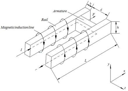
The railgun includes two parallel copper rails across which an armature makes electrical contact (see Fig. 1). The rails are copper strips × and length . The distance between the two rails is . A large current pass through the rails and the armature (projectile), and the projectile current interacts with the strong magnetic fields generated by the rails. It produces a strong force to accelerate the armature together with the projectile along the rails. Meanwhile, a mutually repulsive force occurs between the two rails.
Fig. 1Schematic of railgun
The magnetic force per unit length on the rail is:
The coefficient can be calculated as:
where is the permeability, is the current intensity in the rail, is the thickness of the rail, is the width of the rail, is the distance between the two rails, is one point on the left rail, is one point on the right rail, is the running position of the armature.
Using the regressive interpolation, the nonlinear electromagnetic force can be given as below:
where:
The magnetic force can be expressed in Fourier series form and substituted into the force balance equation of the rail, yields:
where is the modulus of elasticity of the rail material, is the sectional modular of the rail, is the stiffness of the elastic foundation, is the position coordinate in the direction of the rail length, is the length of the rail.
From Eq. (4), the static displacement of the rail can be obtained and the average displacement of the rail can be calculated as:
3. Electromechanical coupled nonlinear dynamics equations of the rail
The dynamic equation of the rail can be given as:
where is the dynamic displacement of the rail, is the mass coefficient per unit length of the rail, is the dynamic electromagnetic force on the rail, is the time.
The dynamic electromagnetic force is:
where:
Substituting Eq. (7) into (6), and letting the nonlinear parameter , yields:
Let , substituting it into Eq. (8), yields:
where:
Let Eq. (9) equal constant , thus:
where .
From Eq. (11), it is known:
where .
From Eq. (12), and the boundary conditions and the continuity conditions of the rail, the natural frequencies and the mode functions of the rail can be obtained.
4. Forced response of the rail to running electromagnetic force
As the electromagnetic force runs along the rail with a constant velocity , it can be expressed as:
Substituting Eq. (12) and (13) into Eq. (6), the generalized force can be given:
The generalized coordinate is:
From Eq. (15), the resonance condition can be obtained:
5. Nonlinear critical velocities
Let:
and:
where is the nonlinear vibration frequency of the rail considering electromechanical coupled effects.
Letting , and Eq. (10) can be changed into following form:
Substituting Eqs. (17) and (18) into (19), and then let sum of the coefficients with the same order power equal zero, following equations can be given:
Here, initial conditions are:
Then, solution of zero order equation under above initial conditions is:
Substituting Eq. (21) into (20b), yields:
In order to remove secular item, let , then:
Substituting Eqs. (21) and (23) into (20c), yields:
In order to remove secular item, let:
then the equation of the magnitude-frequency relationship is:
Combining Eq. (25) with Eq. (16), the critical velocity of the rail running can be obtained:
Assuming that the second projectile is fired when the first projectile leaves just now from the exit, the equivalent initial displacement can be obtained as below.
When the projectile runs to the exit, the real displacements of the rail are given from Eqs. (12) and (15):
From Eq. (27), the equivalent initial displacement for the second projectile to fire can be given:
Eq. (28) gives relationship between the the equivalent initial displacement for the second projectile to fire and the exit velocity for the first projectile. For mode one, Eq. (28) is changed into following form:
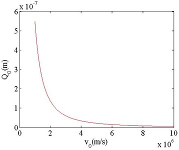
Using Eq. (29), the relationship between the the equivalent initial displacement for the second projectile to fire and the exit velocity for the first projectile is obtained (see Fig. 2). It shows that the equivalent initial displacement decreases with increasing the exit velocity for the first projectile. When the exit velocity is smaller than 2000 km/s, the equivalent initial displacement decreases rapidly with the exit velocity .
Fig. 2Q0 as function of v0
6. Results and discussions
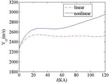
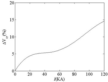
Using above equations, the critical velocity of the railgun system and their changes along with the system parameters are investigated (see Fig. 3). It shows:
1) When the current in the rail grows, the critical velocity of the railgun system grows because of the effects of the electromagnetic force. When the current grows from 0 to 120 KA, the critical velocity increases from 2271 m/s to 2524 m/s.
As the electromagnetic nonlinearity is considered, the critical velocity of the railgun system is increased further. Increasing the current in the rail, the difference between the linear critical velocities and the nonlinear critical velocities becomes large.
When the current grows from 0 to 20 KA, the difference between the linear critical velocities and the nonlinear critical velocities increases significantly. When the current grows from 20 to 50 KA, the difference increases slightly. When the current is above 50 KA, the difference increases significantly with the current again. At 120 KA, the difference between the critical velocities and the nonlinear critical velocities gets to 14.57 %. Therefore, the electromagnetic nonlinearity of the railgun system should be considered when the rail current is relatively large.
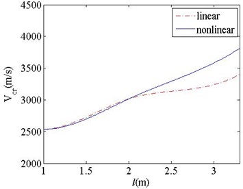
2) When the armature runs along the rails ( grows), the critical velocity of the railgun system increases. Considering the nonlinearity of the railgun system, the critical velocity of the railgun system is almost identical with the linear critical velocity when the armature position is from 0 to 2 m. After 2 m, the nonlinear critical velocity is larger than the linear one, and the difference between the nonlinear and linear critical velocities increases significantly with increasing the position . It shows that the railgun system is a critical velocity changing system caused by the electromagnetic force and the force moving on the rail. For the armature position larger than 2 m, the nonlinearity of the railgun system should be considered.
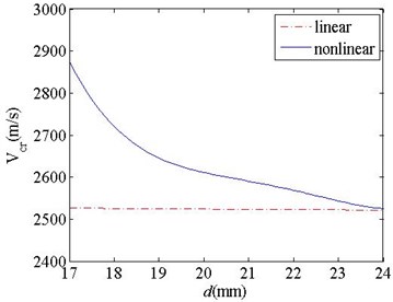
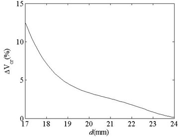
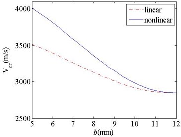
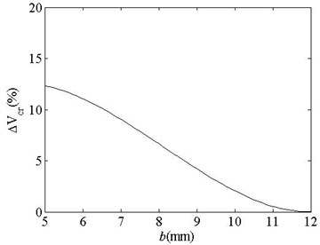
3) When the distance between the two rails increases, the linear critical velocity of the railgun system does not change. As the nonlinearity of the railgun system is considered, the critical velocity of the railgun system increases significantly. When the distance between the two rails is small, the difference between the linear and nonlinear critical velocities is large. At 17 mm, the difference between the linear and nonlinear critical velocities gets to 12.5 %. As the distance between the two rails increases, the difference between the linear and nonlinear critical velocities decreases significantly. The results show that the nonlinearity of the railgun system should be considered for a smaller distance between the two rails.
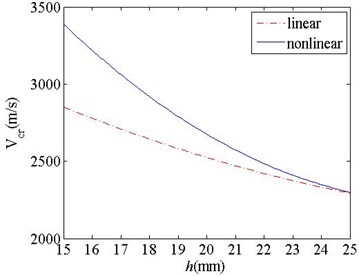
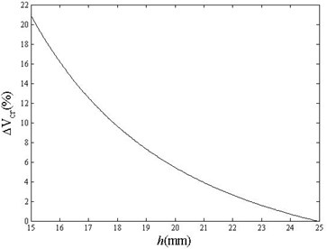
4) When the rail thickness increases, the critical velocity of the railgun system decreases significantly. As the nonlinearity of the railgun system is considered, the critical velocity of the railgun system increases. When the rail thickness is small, the difference between the linear and nonlinear critical velocities is large. When the rail thickness is 0.005 m, the difference between the critical velocities gets to 12.4 %. As the thickness increases, the difference between the linear and nonlinear critical velocities decreases significantly. At 0.012 m, the difference deduces to zero. It shows that the nonlinearity of the railgun system should be considered for a smaller rail thickness .
5) When the rail width increases, the linear critical velocity of the railgun system decreases. As the nonlinearity of the railgun system is considered, the critical velocity of the railgun system increases. When the rail width increases, the difference between the linear and nonlinear critical velocities decreases significantly. For the width of 0.015 m, the difference between the critical velocities gets to 20.8 %. For the width of 0.025 m, the difference between the critical velocities deduces to zero. So, the effects of the nonlinearity of the railgun system on the critical velocity should be considered for a small rail width .
6) When the stiffness of the elastic foundation increases, the linear critical velocity of the railgun system increases gradually. As the nonlinearity of the railgun system is considered, the critical velocity of the railgun system becomes large. As the stiffness increases, the difference between the linear and nonlinear critical velocities decreases gradually. It shows that the nonlinearity of the railgun system should be considered for a smaller stiffness of the elastic foundation.
Fig. 3Nonlinear critical velocities of the railgun system and their changes
a) Critical velocities as function of
b) Velocity difference as function of
c) Critical velocities as function of
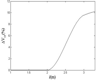
d) Velocity difference as function of
e) Critical velocities as function of
f) Velocity difference as function of
g) Critical velocities as function of
h) Velocity difference as function of
i) Critical velocities as function of
j) Velocity difference as function of
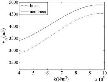
k) Critical velocities as function of
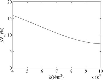
l) Velocity difference as function of
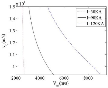
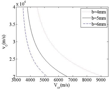
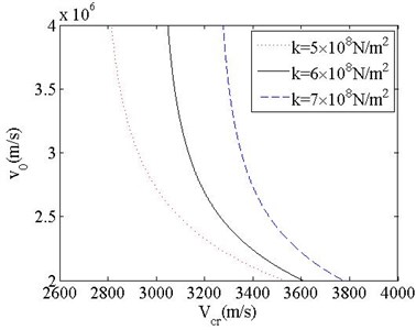
Using Eqs. (26) and (28), the relationship between the nonlinear critical velocity of the projectile and the exit velocity of the last projectile is analyzed (see Fig. 4). These figures show:
1) The nonlinear critical velocity decreases gradually with the exit velocity of the last projectile. It shows that the exit velocity of the last projectile has significant effects on the critical velocity of the next projectile. The effects are related to some system parameters.
2) For a larger current in the rail, the critical velocities of the rail decreases more significantly with the exit velocity of the last projectile. When the rail current is small, the critical velocities of the rail are not nearly influenced by the exit velocity of the last projectile. It is because the electromagnetic nonlinearity is relatively small when the rail current is small.
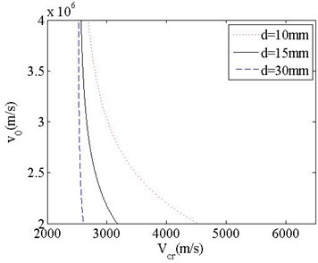
3) When the clearance between two rails is small, the critical velocities of the rail are not nearly influenced by the exit velocity of the last projectile. As the clearance between two rails increases, the critical velocities of the rail decreases significantly with the exit velocity of the last projectile. It is also because the electromagnetic nonlinearity is relatively small when the rail clearance is large.
Fig. 4Relationship between vcr and v0
a) Several
b) Several
c) Several
d) Several
4) As the rail thickness decreases, the critical velocities of the rail decrease more significantly with the exit velocity of the last projectile. It shows that the effects of the electromagnetic nonlinearity are more obvious for a small rail thickness When the electromagnetic nonlinearity is considered, the difference between the critical velocities for the different rail thickness is smaller than that when the electromagnetic nonlinearity is not considered. It shows that the effects of the rail thickness on the critical velocities of the rail become small when the electromagnetic nonlinearity is considered.
5) As the stiffness of the elastic foundation decreases, the critical velocities of the rail decrease more significantly with the exit velocity of the last projectile. It shows that the effects of the electromagnetic nonlinearity are more obvious for a small stiffness . When the electromagnetic nonlinearity is considered, the difference between the critical velocities for the different stiffness is larger than that when the electromagnetic nonlinearity is not considered. It shows that the effects of the stiffness on the critical velocities of the rail become large when the electromagnetic nonlinearity is considered.
In order to illustrate our analytical results, a FEM analysis package, ANSYS, is used to simulate dynamics performance of the railgun system. The FEM model and the mesh-dividing pattern of the railgun system are shown in Fig. 5. The element number of the FEM is 909, and the node number is 5338. The boundary conditions for dynamic simulation of the railgun system are: one end of the rail is fixed, and another end is free, and the rail is supported on the elastic base with the stiffness coefficient 5×10⁸ N/m2.
Using the FEM model, the forced responses of the rail to the running electromagnetic load are simulated. The comparison between the calculative results and the simulated ones are done. The used parameters in simulation are taken to be the same as ones used in analytical calculations above-mentioned.
Fig. 5FEM model of the railgun system
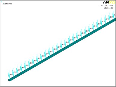
a) FEM model
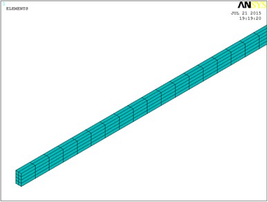
b) Mesh dividing pattern
Fig. 6Comparison between the calculative results and the simulated ones
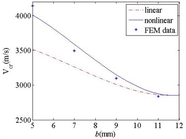
a) Critical velocities as function of
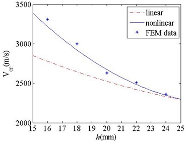
b) Critical velocities as function of
Fig. 6(a) shows the comparison between the calculative critical velocities and the simulated ones for the different rail thickness. Fig. 6(b) shows the comparison between the calculative critical velocities and the simulated ones for the different rail width. Fig. 7(a) gives the dynamic displacements of the rail as a function of the load running velocity for the railgun system with rail thickness of 5 mm. Fig. 7(b) gives the dynamic displacements of the rail as a function of the load running velocity for the railgun system with rail width of 18 mm. Fig. 8(a) gives the dynamic displacement responses of the rail to a given load running velocity at some time for the railgun system with rail thickness of 5 mm. Fig. 8(b) gives the dynamic displacement responses of the rail to a given load running velocity at some time for the railgun system with rail width of 18 mm.
Figs. 6, 7 and 8 show:
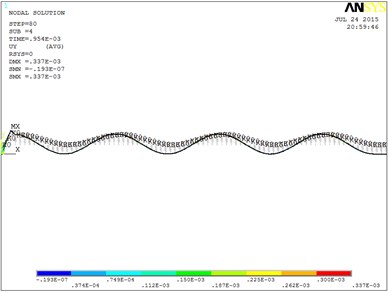
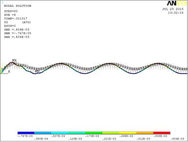
The vibration magnitude of the rail after the armature is much larger than that in front of armature. As the armature runs, the large magnitude vibration range of the rail increases gradually, and the vibration magnitude of the rail increases gradually as well. When the load running velocity gets to the some velocity of the railgun system, the vibration magnitude of the rail gets to the maximum.
Fig. 7Dynamic displacements of the rail as a function of the load running velocity
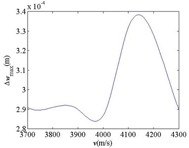
a) 5 mm
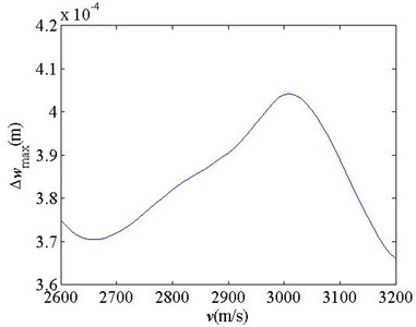
b) 18 mm
Fig. 8Dynamic displacement responses at some time for a given load running velocity
a) 5 mm
b) 18 mm
For the thickness of 5 mm, when the load running velocity gets to 4000 m/s, the dynamic displacements of the rail begin to increase obviously, and gets to the maximum at the load running velocity of 4140 m/s, and then decrease obviously with increasing the load running velocity. So, the critical velocity of the railgun system is 4140 m/s for the railgun system with the thickness of 5 mm.
As the rail thickness increases, the critical velocities of the railgun system decrease significantly. When the thickness is equal to 11 mm, the critical velocity of the railgun system reduces to 2840 m/s.
For the width of 18 mm, when the load running velocity gets to 2700 m/s, the dynamic displacements of the rail begin to increase obviously, and gets to the maximum at the load running velocity of 3000 m/s, and then decrease obviously with increasing the load running velocity. So, the critical velocity of the railgun system is 3000 m/s for the railgun system with the width of 18mm. It should be noted that the sensitivity of the dynamic displacements of the rail on the rail width is smaller than that on the rail thickness. As the rail width increases, the critical velocities of the railgun system decrease significantly as well. When the width is equal to 24 mm, the critical velocity of the railgun system reduces to 2360 m/s.
From Figs. 6, 7 and 8, it is known that the FEM simulated critical velocities of the railgun system is near to ones calculated by the nonlinear analytical equations. Here, the FEM simulated critical velocities are in good agreement with ones calculated by the nonlinear analytical equations, and the maximum error between them is 3.2 %. The results illustrate the analytical results about critical velocities of the railgun system in this paper.
It should be noted that the errors between the FEM simulated critical velocities and the analytical calculated ones increase with decreasing the rail thickness or the rail width. It is because only the first order nonlinear term is considered in our analytical Eq. (8). As the rail thickness or the rail width decrease, the nonlinearity of the railgun system increases, so the errors between the FEM simulated critical velocities and the analytical calculated ones increase.
For the thickness of 5 mm, the maximum error between the FEM simulated critical velocities and the ones calculated by the nonlinear analytical equations is 3.2 % as above stated. For the thickness of 11 mm, the error between them is 1.3 %. When the rail width increases from 16 mm to 24 mm, the error between them decreases from 2.3 % to 0.5 %. Therefore, for the stronger nonlinear dynamics problem with smaller rail thickness and smaller rail width, in order to reduce the analytical calculated errors, more order nonlinear terms can be considered for a stronger nonlinear dynamics problem.
7. Conclusions
In this paper, the nonlinear electromechanical coupled dynamics equations for the railgun are proposed. Based on it, the equation of the nonlinear critical velocity of the projectile is given and the effects of the electromagnetic nonlinearity on the critical velocity of the projectile are investigated. The effects of the projectile exit velocity on the nonlinear critical velocity are studied. Results show:
1) The critical velocity of the railgun system increases when the electromagnetic nonlinearity is considered.
2) The nonlinear critical velocity is influenced by the system parameters such as rail current, rail thickness, rail distance, etc. Increasing the rail current, the difference between the linear and nonlinear critical velocities becomes large.
3) The railgun system is a critical velocity changing system. For large armature position, the nonlinearity of the railgun system should be considered.
4) As the distance between the two rails or the rail thickness increases, the difference between the linear and nonlinear critical velocities decreases significantly. It shows that the nonlinearity of the railgun system should be considered for a smaller distance between the two rails and a smaller rail thickness.
5) The nonlinear critical velocity decreases gradually with the exit velocity of the last projectile. It shows that the exit velocity of the last projectile has significant effects on the critical velocity of the next projectile.
References
-
Fair H. Progress in electromagnetic launch science and technology. IEEE Transactions on Magnetics, Vol. 43, Issue 1, 2007, p. 93-98.
-
Shvetsov G., Rutberg P., Budin A. Overview of some recent EML research in Russia. IEEE Transactions on Magnetics, Vol 43, Issue 1, 2007, p. 99-106.
-
Lehmann P., Peter H., Wey J. First experimental results with the ISL 10-MJ-DES railgun PEGASUS. IEEE Transactions on Magnetics, Vol. 37, Issue 1, 2001, p. 435-439.
-
Fryba L. Vibration of Solids and Structures under Moving Loads. Noordhoff, Gronningen, the Netherlands, 1977.
-
Tzeng J. T. Dynamic response of electromagnetic railgun due to projectile movement. IEEE Transactions on Magnetics, Vol. 39, Issue 1, 2003, p. 472-475.
-
Tzeng J. T., Sun W. Dynamic responce of cantilevered rail guns attributed to projectile/gun interaction – theory. IEEE Transactions on Magnetics, Vol. 43, Issue 1, 2007, p. 207-213.
-
Nechitailo N. V., Lewis B. K. Critical velocity for rails in hypervelocity launchers. International Journal on Impact Engineering, Vol 33, Issues 1-12, 2006, p. 485-495.
-
Johnson A. J., Moon F. C. Elastic waves and solid armature contact pressure in electromagnetic launchers. IEEE Transactions on Magnetics, Vol. 42, Issue 3, 2006, p. 422-429.
-
Johnson A. J., Moon F. C. Elastic waves in electromagnetic launchers. IEEE Transactions on Magnetics, Vol. 43, Issue 1, 2007, p. 141-144.
-
Tumonis L., Schneider M., Kacianauskas R., Kaceniauskas A. Structural mechanics of railguns in the case of discrete supports. IEEE Transactions on Magnetics, Vol. 45, Issue 1, 2009, p. 474-479.
-
Xu L., Geng Y. Dynamics of rails for electromagnetic railguns. International Journal of Applied Electromagnetics and Mechanics, Vol. 38, Issue 1, 2012, p. 47-64.
-
He W., Bai X. Dynamic responses of rails and panels of rectangular electromagnetic rail launcher. Journal of Vibration and Shock, Vol. 32, Issue 1, 2013, p. 44-148, (in China).
-
Christian S., Liudas T., Rimantas K. Experimental and numerical investigations of vibrations at a railgun with discrete supports. IEEE Transactions on Plasma Science, Vol. 41, Issue 5, 2013, p. 1508-1513.
-
Geng Y. Electromechanical coupled dynamics of rails for electromagnetic launcher. International Journal of Applied Electromagnetics and Mechanics, Vol. 42, Issue 3, 2013, p. 369-389.
-
Xu L., Zheng F., Peng L. Electromechanical coupled nonlinear free vibration of rails for electromagnetic railguns. International Journal of Applied Electromagnetics and Mechanics, Vol. 47, Issue 2, 2015, p. 313-322.
About this article

This project is supported by the Doctoral Research Program Foundation of Education Ministry of China (Priority development areas, No. 20131333130002).
