The prediction of vibration and noise for the high-speed train based on neural network and boundary element method

The prediction of vibration and noise for the high-speed train based on neural network and boundary element method

1. Introduction

2. Multi-body dynamics model of the high-speed train

3. Neural network

4. Verification and analysis of NARX NN model

5. Numerical computation and verification of low frequency noise for the high-speed train

6. Conclusions

4.1. Data acquisition

4.2. Network training and model verification

5.1. Numerical computation of the low frequency noise for the high-speed train

5.2. Experimental verification of the low frequency noise for the high-speed train

Abstract

References

About this article

Qian, Kun; Liang, Jie; Gao, Yin-han

Journal of Vibroengineering

Browse Journal

Submit article

Published: 30 December 2015

Check for updates

Kun Qian¹

Jie Liang²

Yin-han Gao³

^{1, 2, 3}State Key Laboratory of Automotive Simulation and Control, Jilin University, Changchun, Jilin Province, 130022, China

Corresponding Author:

Jie Liang

Cite the article Download PDF

Downloads 1493

The vibration acceleration of the high-speed train is an important parameter reflecting the state of track irregularities and the quality of contact between wheel and rail. A model for predicting vibration acceleration of the high-speed train based on nonlinear auto-associative neural network (NARX NN) and multi-body dynamics model is built. In order to improve the prediction precision, the parameters such as the order of time-delay and hidden nodes are determined by traversal method. The vibration acceleration computed by the NN model is then compared with that computed by SIMPACK model. The corresponding results show that the output of NARX NN is highly consistent with those of the multi-body dynamics model. Then, the vibration acceleration computed by NN model is used to compute the low frequency noise of the high-speed train. The computational results are also compared with those of the experimental values, and they are consistent with each other. It shows that the computational noises are reliable, and it also indirectly indicates that the vibration acceleration predicted by NN model is credible. Otherwise, the computational results will deviate far away from the experimental value.

The vibration response of the high-speed train comes from track irregularities, and is vital to reflect the ride comfort and safety. Several parameters such as Diekemann, Sperling, L/V ratio are used as rules to evaluate the ride comfort and running safety according to the computational results.

However, there is still lack of effective measures to evaluate the vibration response of a running train with high reliability. Actually, testing requires a lot of manpower and costs due to the great amount of existing trains. The track quality index (TQI) which is computed based on measurement data of track irregularities is a traditional method to evaluate the track irregularities. As a result, it provides the same guidance for all different types of train due to the single standard. Building dynamics model of track-train system is another method to evaluate the irregularities. For example, with the input of track irregularities, the train body vibration accelerations were predicted according to the dynamic method[1]. Zuo [2] built the vertical vibration model of the train body using differential equations, and the train vibration response was obtained by employing the multi-dynamics software SIMPACK. However, the parameters and equivalent treatments of the train system will directly affect the computational precision. As a result, a very accurate dynamic model is also difficult to obtain the acceptable results.

In recent years, the modeling methods of track-train system based on the commercial software have attracted a lot of attentions [3]. Pan [4] predicted reduction rate of wheel loads accurately using NN based on track irregularities. Chen [5] verified the modeling method of NN based on the measured data. TTCI technology centers predicted the wheel/rail force using the NN method with many kinetics parameters as the input[6, 7].

In this paper, the prediction model of the train vibration is built using NN technique regarding track irregularities as the input and the train vibration acceleration as the output of the model, respectively. A track-train dynamic system is built based on SIMPACK software to obtain large amounts of data for NN model training. The vibration acceleration computed by NN is then compared with that computed by SIMPACK. The results show that the output of NARX NN is highly consistent with that of the multi-body dynamics model. Then, the vibration acceleration computed by NN is used to compute low frequency noise of the high-speed train. The computational results are also compared with those of the experimental values, and they are consistent with each other. It shows that the computational noise is reliable, and it also indirectly indicates that the vibration acceleration predicted by NN is credible. Otherwise, the computational results will deviate far away from the experimental values.

To investigate the influence of track irregularities on the train running, some researchers simulated the vibration response under track irregularities by building the simulation model based on SIMPACK.

SIMPACK is the commercial software, which can be used to simulate the running state of the high-speed train. Firstly, the global coordinate system should be built, and the corresponding geometric parameters of the wheels should be also set. Secondly, the relationship between the wheel and rail should be defined, and a simplified contact model is adopted. The interaction force between the wheel and rail is determined based on Herzian contact theory.

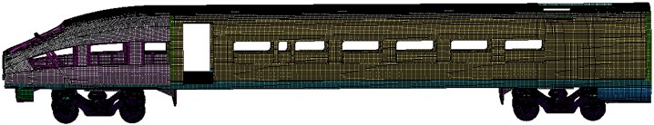
Based on the corresponding geometric model, bogies, wheels, axle boxes and the body are modeled in SIMPACK, respectively. The corresponding parameters and model has been obtained as shown in Table 1 and Fig. 1, respectively [8].

Table 1Mainly structural parameters of the multi-body dynamics model [8]

Train body mass	38 t	Center of gravity for train body	1.656 m
Frame mass	2056 Kg	Center of gravity for frame	–0.52 m
Wheels mass	1627 Kg	Body rolling inertia	114.4 t∙m²
Primary suspension stiffness	886 KN/m	Body nutation inertia	1730 t∙m²
Secondary suspension stiffness	195 KN/m	Body shaking inertia	1632 t∙m²

Fig. 1Multi-body dynamics model of the high-speed train [8]

NN adopted in this paper is different from the multi-body dynamics model. It does not need to consider the structural parameters and simplify the model. It can improve the prediction precision by setting up a reasonable arrangement for the network structure. In NN model, taking the irregularity as the input and vibration acceleration as the output, NN model is then built, which is corresponding to the multi-body dynamics model.

NARX NN has been widely used in the field of system modeling due to its approximation and generalization ability for nonlinear system. NARX NN structure can be divided into four layers including input layer, delay layer, hidden layer and output layer. The basic structure is shown in Fig. 2. The input layer is responsible for receiving signals instead of computing. The node of time-delay layer is considered as a multi-step delay operator, and determines the time-delay order of the input signal and output feedback signal, while the time-delay signals are transferred to the output layer after nonlinear processing through hidden layer nodes. According to the above analysis, the final output is obtained through linear weighted method [9].

Fig. 2Structure of NARX NN

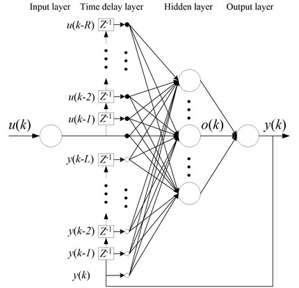
If $R$ is the input time-delay step and $L$ is the output delay step, the network input is then defined as follows:

1

u (k) = [u (k), . . ., u (k - R), y (k), . . ., y (k - L)] .

The output of the $i$ th hidden layer nodes is presented as follows:

2

o (k) = f_{N 1} (u (k) w_{N 1} + b_{N 1}),

3

y (k) = f_{N 2} (o (k) w_{N 2} + b_{N 2}),

where $u,$ $y,$ and $o$ represent $P$ -dimension input vector, $Q$ -dimension output vector and $N$ -dimension hidden layer nodes, respectively. $R$ is also delay order. $L$ is the output delay order. $b_{N 1}$ is the threshold of the input layer, and $b_{N 2}$ is the threshold of hidden layer. $w_{N 1}$ and $w_{N 2}$ are the connection weights of delay layer to hidden layer, and hidden layer to output layer, respectively. $f_{N 1}$ is the transfer function of hidden layer neurons, and $f_{N 2}$ is the activation function of the output layer.

The Bayesian regularization (BR) algorithm, which references correction coefficient, is used in NARX NN, and the evaluation function of is given as follows:

4

F (w) = α E_{w} + β E_{D},

5

E_{w} = \frac{1}{m} \sum_{e = 1}^{m} w_{e}^{2},

6

E_{D} = \frac{1}{n} \sum_{f = 1}^{n} (t_{f} - y_{f})^{2},

where $E_{w}$ is the network mean square value of all weights. $m$ is the total number of network weights, $w_{e}$ is the network weights of group $e$ . $n$ is the total number of training value. $t_{f}$ is the desired training output of group $f$ . $y_{f}$ is the network training output of group $f$ . $α$ and $β$ are the regularization coefficients and adaptively controlled by BR algorithm in the case of training NN. If the time $α$ and $β$ are optimal, and the network training also achieves the optimal solution. Finally, the optimal solution of $α$ and $β$ is $α = γ / 2 E_{w} (w_{0}),$ $β = m - γ / 2 E_{D} (w_{0}) .$ $w_{0}$ is minimum point, $γ$ is the effective number of network parameters.

NARX NN prediction model of the vibration is built in this paper by taking the input $u (t)$ as the track irregularity parameters, and the model output $y (t)$ as the vibration acceleration. The purpose of accurately predicting the vibration acceleration is to train the network using BR algorithm through reasonably setting NN delay order and hidden layer.

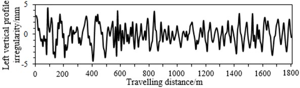
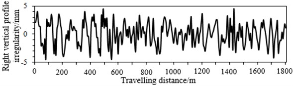
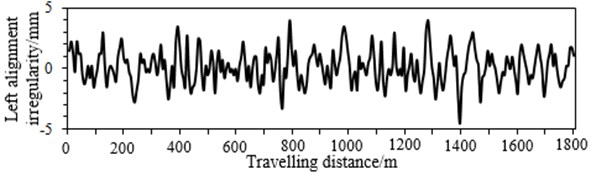
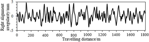
Fig. 3Model input data

a)

b)

c)

d)

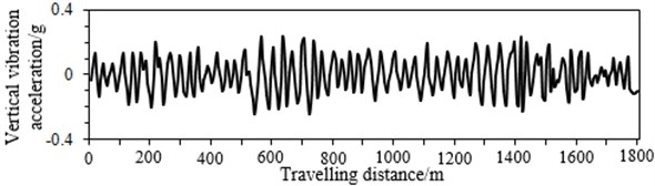
In this paper, the input and output data generated from the multi-body dynamics model are used to verify NN model. When we select track irregularities as the input, considering the track cross-level and gauge irregularity can be computed through the left vertical profile irregularity, right vertical profile irregularity, left alignment irregularity and right alignment irregularity. Therefore, they are elected as the input, as shown in Fig. 3. The vertical vibration acceleration is the main factor which influences ride comfort and stability. Therefore, taking the vertical vibration acceleration as an example, we extract 1800 m travelling distance from the multi-body dynamics model. Among which, the first 1300 m is taken as the training data, and the final 500 m is taken as the verified data, as shown in Fig. 4.

Fig. 4Model output data

In order to describe the prediction effect of NN model, coefficient $R$ and RMSE are applied to evaluate the prediction performance of NN model. The computational formulas are shown as Eq. (7) and Eq. (8):

7

R (d, y) = \frac{\sum_{i = 1}^{N} (d (i) - \bar{d}) (y (i) - \bar{y})}{\sqrt{\sum_{i = 1}^{N} {(d (i) - \bar{d})}^{2}} \sqrt{\sum_{i = 1}^{N} (y (i) - \bar{y})^{2}}},

8

R M S E (d, y) = \sqrt{\frac{1}{N} \sum_{i = 1}^{N} (d (i) - y (i))^{2}},

where, $d$ is the target value of the vibration acceleration simulated by using SIMPACK model. $y$ is the output value predicted by NN model. $N$ is the size of samples. $R$ is correlation coefficient. The greater the $R$ , the closer the SIMPACK simulation output and NN output are. The smaller the RMSE, the higher the network output precision, the better the prediction performance is.

Table 2Structural parameters of NN model

Network type	Hidden nodes number	Time delay step	Training time
NARX	20	25	15

The network training state and prediction performance require to be considered when determining the model parameters, such as time-delay order, hidden nodes number, training time and so on. If the size of hidden nodes is too small, it is difficult to ensure the network accuracy. If the size of hidden nodes is too big, network generalization capability will be decreased. So, the traversal method is regarded as the best method to determine the size of hidden nodes. The network is trained choosing the different size of hidden nodes. Then, the size of hidden nodes with the best performance can be obtained. In this paper, the network structural parameters are identified using the traversal method, as shown in Table 2.

Before prediction, NN model should be trained to build a certain response mechanism. When the input parameters are changed, NN will output the corresponding values. The training sample should be reasonable, which should reflect the whole change trends, and the sample points should include the whole parameter range. In this paper, the vertical vibration acceleration of the high-speed train is obtained using the multi-body dynamics model. According to Fig. 4, it can be seen that the vibration acceleration of the high-speed train can reflect the change trends of the whole travelling process within the first 1300 m. Therefore, the vibration acceleration of the first 1300 m is used to train NN model.

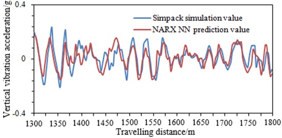
When NN model is trained, the sample data is normalized to eliminate errors caused by the data. The error curve of the network training is shown in Fig. 5. As can be seen from the figure, the network has reached the accuracy requirements after 98 steps training. At this moment, NN model can be used to predict the vertical vibration acceleration of the high-speed train between 1300 m and 1800 m, and the computational results are compared with those of the multi-body dynamics model, as shown in Fig. 6.

As can be seen from Fig. 6, the vibration acceleration of the high-speed train predicted using NN model is very close to those of the multi-body dynamics model. This indicates that NN model can effectively predict the vibration acceleration of the high-speed train.

Fig. 5Error curve of the neural network training

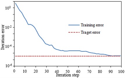
Fig. 6Comparison of the computational results between NN and the multi-body dynamics

The mechanical vibration of the high-speed train will generate a certain noise. As a result, the riding comfort will be reduced, especially in the low frequency. The noise caused by the mechanical vibration is dominant, and the noise caused by the fluid can be neglected. As shown in Fig. 7, the noise distribution of the high-speed train in the low frequency is measured by experiments [10]. It can be seen in the front part of the high-speed train that the noise is mainly caused by the mechanical vibration of bogies and wheels. In this paper, the vibration acceleration of the high-speed train obtained by the multi-body dynamics model and NN model comes from bogies and wheels. Therefore, based on the vibration acceleration of the above prediction, the low frequency noise in the front part of the high-speed train can be computed. Currently, for the low frequency noise, a more effective method to solve this problem is the finite element and boundary element method. Because the high-speed train model is relatively larger with a lot of meshes, it will take a long time using the finite element method to compute it. In addition, the performance of the computer is also very high. Thus the boundary element method is used to compute the low frequency noise of the high-speed train.

Fig. 7Low frequency noise distribution of the high-speed train

The boundary element method is used to compute the low frequency noise in the high-speed train. Firstly, the finite element meshes of the high-speed train must be built. Then, the surface meshes are extracted to obtain the boundary element meshes. Finally, the finite element and boundary element meshes are coupled to compute the internal noise of the high-speed train.

The high-speed train which is principally made of bogies, driver’s cab and the passenger compartment, is complicated. Concretely, the train body, with hollow extruded sections covered as a whole, is constituted by the under frame, the side walls and the roof, where the under frame is made up of the floor, the side girder, the sleeper beam, the traction beam and the buffer beam. Besides, the floor, the side girder, the roof and the side wall are welded by hollow extruded sections with enough rigidity. The aluminum alloy 6N01 with favorable extruding property and welding performance, and the end wall is assembled and welded by aluminum alloy sections.

For the finite element meshes, the unnecessary elements such as chamfers and bolted holes are ignored in order to save the computational time. Concretely, finer meshes are adopted for the key analysis parts and sparser ones for the others. As a result, the mesh quantity can be decreased, and the computational speed can be also improved. The body plates are divided into meshes using shell elements, and the finite element meshes is shown in Fig. 8. It has 452963 elements and 512398 nodes, and most of elements are quadrilateral, with triangular elements at some positions. In addition, bogies are an irregular structure, and the thickness of the cross section is relatively large. Therefore, the tetrahedral element is used to divide the model, as shown in Fig. 9(c), and there are 236801 elements and 329853 nodes. Besides, the density is defined as 2686 kg/m³. The elastic modulus is defined as 72.4 GPa and Poisson ratio is defined as 0.3.

Fig. 8Finite element meshes of the high-speed train

As can be seen from Fig. 8, the finite element meshes of the high-speed train include bogies and wheels. Such model is consistent with the multi-body dynamics model in Fig. 1. However, in the published papers, wheels, bogies and other accessories are both neglected when the finite element model of the high-speed train is built. The mass of bogies and wheels is very big, which will have a relatively large influence on the vibration and noise of the high-speed train. Therefore, if we do not consider bogies and wheels, the computational results will have a certain error.

Fig. 9Local structure meshes of the high-speed train

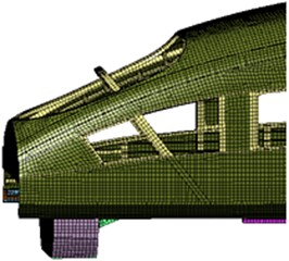
a) Local meshes of the body

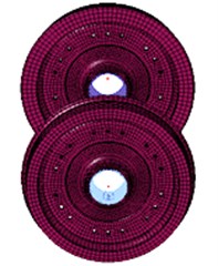
b) Wheel meshes

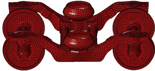
c) Bogie meshes

Fig. 10Boundary element mesh model of the high-speed train

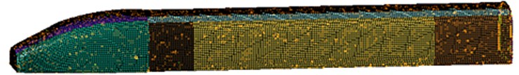
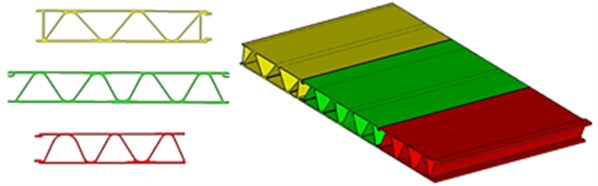
Fig. 11Main structure of the high-speed train

Based on the finite element meshes, the corresponding surface meshes are extracted to build the boundary element meshes, as shown in Fig. 10. The boundary element meshes basically adopts the quadrilateral element, and there are 102358 elements and 123698 nodes. The boundary element meshes are then coupled with the finite element meshes. After that, the vibration acceleration computed by NN model is imported into the coupling model. Finally, the noise in the front part of the high-speed train can be obtained, as shown in Fig. 15.

The computational sound pressure in Fig. 16 is relatively smooth, which can be explained from the following aspects.

The model in Fig. 11 is the main structure of the high-speed train. It mainly has three characteristic cross sections, and the angle of sound-bridge is changing from 55° to 60°. In addition, it can be seen that the structure of sound-bridge is periodic. According to the theory of Photonic Crystals, the periodic structure has a good effect on the low frequency noise. Therefore, the noise peaks of the high-speed train can be weakened, making the curve relatively smooth.

Fig. 12Sound-bridge of the main structure for the high-speed train

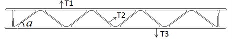
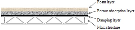
Fig. 13The covering layer structure of the main structure

The acoustic performance of the main structure for the high speed train is seriously affected by sound-bridge. Therefore, the structure of sound-bridge is researched in this paper. As shown in Fig. 12, when sound-bridge thickness is unchanged, the angle is changed, and the corresponding results are shown in Table 3. As can be seen from Table 3, with the increase of the angle of sound-bridge, the modes of the main structure gradually decrease. The angle of sound-bridge is between 55° and 60°. Therefore, the modes of the main structure are very few, which make noises relatively smooth.

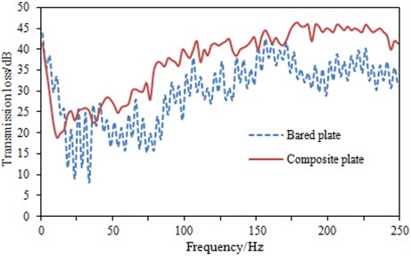
In addition, the main structure of the high-speed train will be covered some other structures. As shown in Fig. 13, damping layer is applied on the surface of the main structure, and then through the porous absorption layer, it is finally connected with foam layer. The sound insulation performance of the main structure is then computed. It is compared with that of the main structure which has a small sound-bridge angle and is not covered any other layers, as shown in Fig. 14. As can be seen from Fig. 14, there are a little peaks in the main structure which has been covered several other layers.

Fig. 14Comparison of transmission loss between two kinds of structures

According to Fig. 15, the noise in the front part of the high-speed train increases when the frequency is increasing. Sound pressure on the surface of the high-speed train at 20 Hz, 150 Hz and 200 Hz is extracted, as shown in Fig. 16. As can be seen from Fig. 15, the maximum sound pressure is at 200 Hz. Sound pressure contour on the surface of the high-speed train in Fig. 16 can further describe this problem. To some extent, it can be shown that the noise of the high-speed train computed is reliable.

Table 3Results under different angles for sound-bridge

Fig. 15Interior noise in the front part of the high-speed train

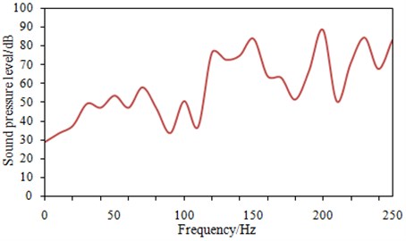
Fig. 16Sound pressure contour of the high-speed train at several frequency points

a) Sound pressure contour of the high-speed train at 20 Hz

b) Sound pressure contour of the high-speed train at 150 Hz

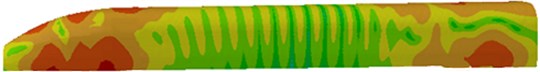
c) Sound pressure contour of the high-speed train at 200 Hz

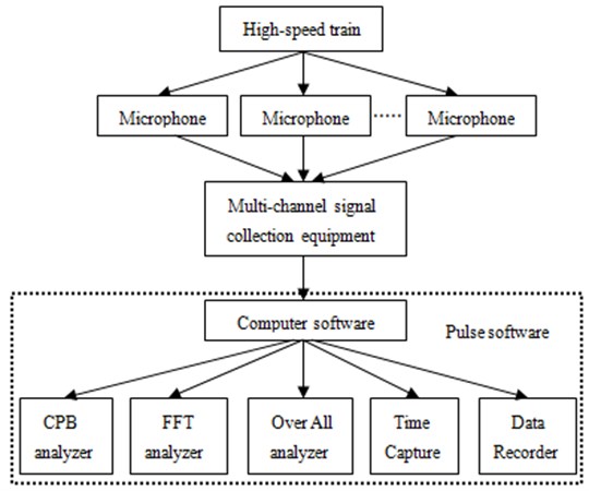
The numerical computation of the vibration acceleration and noise for the high-speed train is a very complicated process, so it is necessary to be verified by means of experiments. Therefore, this paper takes the real train as the object to test its noise. When the wind speed is less than 2 km/h, the noises in the front part of the high-speed train are tested, and layout of testing points is shown in Fig. 17. The test procedure is also shown in Fig. 18. Pulse software which is made by B&K Company is used to test noise of the high-speed train. MPA 201 microphone is adopted to obtain the original signals. Multi-channel collection equipment is used to obtain signals of microphone. Then, the time domain signals can be obtained, as shown in Fig. 19. They are processed in Pulse to obtain the corresponding frequency domain. Finally, the experimental results are compared with the numerical computation results in Fig. 15, as shown in Fig. 20.

Fig. 17Testing point of noise in the front part for the high-speed train

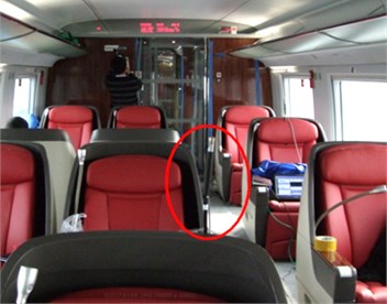
Fig. 18Testing process in the front part of the high-speed train

As can be seen from Fig. 20, the experimental values are also smooth. On one hand, it can be explained from the above analysis. On the other hand, the results of time domain can also explain this question as follows. In this paper, the frequency domain results researched are only within 250 Hz, which correspond to the time domain results within 0.5 s in Fig. 19. As can be seen from Fig. 19, within 0.5 s, the noise peaks are indeed little. The noise peaks are significantly higher in the middle and high frequency range over 250 Hz. Therefore, the curve in the paper is relatively smooth.

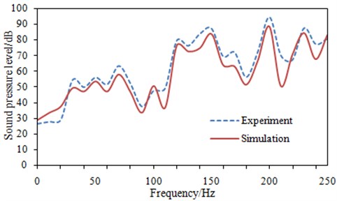
In addition, as can be seen from Fig. 20, the change trends and sizes between experiment and simulation are both very close. The experimental values are always larger than the simulation results, which is mainly due to the experimental results including the air flow noise. It can also be seen that the air flow noise at the low frequency is very small. Therefore, it is feasible to ignore the flow noise, and it can be used to predict the noise in the front part of the high-speed train. The numerical computation is based on the vibration acceleration computed by NN model. Therefore, when the noises between experiment and simulation are consistent with each other, it also indirectly indicates that the vibration acceleration predicted by NN model is reliable. Otherwise, the computational noises will deviate far away from the experimental values.

Fig. 19Time domain of sound pressure for the high-speed train

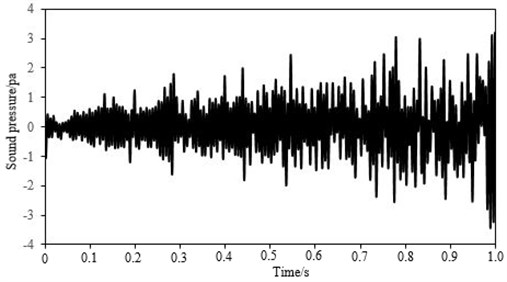
Fig. 20Comparison of noises between experiment and simulation

In this paper, a model for predicting vibration acceleration of the high-speed train based on nonlinear auto-associative neural network (NARX NN) and multi-body dynamics model is built. In order to improve the prediction precision, the parameters such as the order of time-delay and hidden nodes are determined by traversal method. The vibration acceleration computed by the NN model is then compared with that computed by SIMPACK model. The corresponding results show that the output of NARX NN is highly consistent with those of the multi-body dynamics model. Then, the vibration acceleration computed by NN model is used to compute the low frequency noise of the high-speed train. The computational results are also compared with those of the experimental values, and they are consistent with each other. It shows that the computational noises are reliable, and it also indirectly indicates that the vibration acceleration predicted by NN model is credible. Otherwise, the computational results will deviate far away from the experimental values.

Cui Shengai Research on Vehicle Bridge Coupling Vibration Simulation Based on Multi-Body System Dynamics and Finite Element Method. Southwest Jiaotong University, 2009.

Search CrossRef
Zuo Yanyan, Chang Qingbin, Geng Feng, et al. Simulation of vehicle vibration with excitation of rail height irregularity. Journal of Jiangsu University, Vol. 32, Issue 6, 2011, p. 647-651.

Search CrossRef
Yan Hongying, Li Chunqing Research of intelligent simulation forecasting methods on MBR membrane fouling. Computer Measurement and Control, Vol. 21, Issue 8, 2013, p. 2177-2180+2190.

Search CrossRef
Pan Lisha, Cheng Xiaoqing, Qin Yong, et al. Predicting reduction rate of wheel load based on NARX neural network. Urban Mass Transit, Vol. 50, Issue 9, 2012, p. 4-7.

Search CrossRef
Chen Hao, Cheng Xiaoqing, Yu Xiulian, et al. Research on accurate prediction method of train derailment coefficient. Computer Simulation, Vol. 30, Issue 7, 2013, p. 142-146.

Search CrossRef
Li K. H. D., Medah A., Kalay S. Development and implementation of performance-based track geometry inspection technology. Railway Engineering Eight International Conference on Maintenance and Renewal of Permanent War: Power and Signaling; Structures and Earthworks, Engineering Technical Press, 2005.

Search CrossRef
Guins D., Kalay S. Performance-based track geometry assessment for network efficiency. International Conference on Heavy Haul Association, Specialist Technical Session, 2003.

Search CrossRef
Liu C. Y., Wang T. H., Bo Z. Z., et al. Internal low-frequency noise analysis of high-speed train under mechanical excitation. Journal of Vibroengineering, Vol. 16, Issue 6, 2014, p. 3086-3095.

Search CrossRef
Han Liqun Artificial Neural Network Tutorial. Beijing Institute of Posts and Telecommunications Publishing House, 2006.

Search CrossRef
Zhang Jie, Xiao Xinbiao, Han Jian, et al. Characteristics of noise distribution at the ends of the coach and acoustic modal analysis of high-speed train. Journal of Mechanical Engineering, Vol. 50, Issue 12, 2014, p. 97-103.

Search CrossRef

Basic size

$T_{1} =$ 4 mm, $T_{2} =$ 2.5 mm, $T_{3} =$ 3 mm

Sound-bridge angle

Sound-bridge number

Modal number

Received

21 March 2015

Accepted

16 August 2015

Published

30 December 2015

SUBJECTS

Vibration in transportation engineering

Keywords

neural network

multi-body dynamics model

track irregularity

vibration acceleration

low frequency noise

This is an open access article distributed under the Creative Commons Attribution License, which permits unrestricted use, distribution, and reproduction in any medium, provided the original work is properly cited.