Development and verification of time-dependent bounding surface model under metro dynamic loads

Luo, Junhui; Miao, Linchang; Li, Renjue; Shi, Wenbo; Chen, Yinan; Yan, Bo

Journal of Vibroengineering

Browse Journal

Submit article

Published: 30 December 2015

Check for updates

Development and verification of time-dependent bounding surface model under metro dynamic loads

Junhui Luo¹

Linchang Miao²

Renjue Li³

Wenbo Shi⁴

Yinan Chen⁵

Bo Yan⁶

^{1, 2, 4, 5}Institute of Geotechnical Engineering of Southeast University, Nanjing 210096, China

³Changzhou Institute of Technology, Changzhou 213002, China

⁶Research and Design Institute of Urban Rail Transit of Jiangsu Province, Nanjing 210008, China

Corresponding Author:

Linchang Miao

Cite the article Download PDF

Downloads 1262

Abstract

To study the dynamic characteristics of soft soil foundation under the long-term metro dynamic loads, modified model based on the bounding surface model was presented. The Mesri creep formula was introduced into the bounding surface model, then it could not only consider the effects of time but also could describe the soil’s arbitrary shear stress levels. The modified bounding surface model was derived using the Newton-Raphson method and the secondary development of the model was conducted. Meanwhile, in order to verify the model, the dynamic triaxial tests of the soft soil were conducted by GDS dynamic triaxial equipment and the metro dynamic loads were simulated during dynamic triaxial tests. Then, the numerical simulation of modified bounding surface model was carried out for soft soil and the numerical results were compared with the test results. The results show that the time-dependent bounding surface model provides a more accurate calculation for the dynamic strain, and establishes a theoretical foundation for predicting the settlement of the soft soil.

1. Introduction

Bjerrum was the first scholar to research on the soft soil and proposed the concept of total strain decomposition [1]. It was found that the soft soil area has high compression, high water content, low permeability, creep engineering properties. The soft soil foundation will produce greater amounts of long-term settlement in the subway given the vibration occurring as a result of the moving loads [2]. In order to more accurately calculate the settlement of soft soil during subway vibration operation, it is necessary to establish a dynamic constitutive model consideration time effects under dynamic loads [3].

Current plastic models typically employ the bounding surface model to study dynamic soil characteristics. Dafalias proposed the mathematic expression of the bounding surface model [4-6]. Compared with the cam-clay model, the bounding surface model could better describe the plastic hysteresis characteristics of the soil in calculations of the dynamic strain-stress soil relations under the dynamic loads [7, 8]; consequently, it was often used to analyze dynamic problem [9, 10].

The creep empirical model has two types: Singh-Mitchell and the Mesri creep model. The former model can only be calculated for the 20 %-80 % range of the shear stress level and Mesri model improved this problem [11-13]. Then numerous studies on the creep empirical model under dynamic loads have been carried out [14, 15]. However, these studies are not suitable for the numerical simulation analysis of soil settlement under dynamic loads.

Along with these problems, studying the dynamic characteristics and settlement of soft soil foundation under long-term vibration, this paper introduces the Mesri creep model into the boundary surface model. A time-dependent boundary surface model was developed to describe soil creep for arbitrary shear stress levels. Meanwhile, in order to verify the model, the dynamic triaxial tests of the soft soil were conducted and the subway metro dynamic load modes was simulated during the dynamic triaxial tests. Then, the modified bounding surface model was used to simulate for soft soil and the numerical results were compared with the test results. The study of soft soil characteristics under metro dynamic loads provides a theoretical foundation for subsidence prediction.

2. Establishment of the time-dependent bounding surface model under dynamic loads

The modified bounding surface model was derived on the basis of the rheological model, the yield criterion, hardening law and flow rule. Based on the incremental theory [16, 17], the total strain $d ε_{i j}$ is divided into the sum of three partial strain increments:

1

d ε_{i j} = d ε_{i j}^{e} + d ε_{i j}^{p} + d ε_{i j}^{t},

where $d ε_{i j}^{e}$ is the elastic strain increment; $d ε_{i j}^{p}$ is the plastic strain increment; and $d ε_{i j}^{t}$ is the creep increment.

2.1. Creep increment

The creep increment is divided into volumetric creep and deviatoric stress creep:

2

d ε_{i j}^{t} = \frac{d ε_{v}^{t}}{3} + d ε_{s}^{t} \frac{d e_{i j}}{q},

where $d ε_{v}^{t}$ is volumetric creep increment; $d ε_{s}^{t}$ is the deviatoric stress creep; and $d e_{i j}$ is the partial strain.

2.1.1. Deviatoric stress creep

Deviatoric stress creep is based on the Mesri creep model. The Mesri model was created as an improvement on the classic Singh-Mitchell creep model. The Singh-Mitchell creep model can only describe 20 %-80 % of soil creep properties for shear stress levels, and when the shear stress level is equal to zero, the strain calculation results are less than zero. For this problem, the Mesri model had been improved to calculate the soil creep under arbitrary shear stress levels.

According to the Singh-Mitchell creep formula:

3

d ε_{s}^{t} = A e^{\bar{α} \bar{D}} {[\frac{(t)_{i}}{t}]}^{m} d t,

where $A$ , $\bar{α}$ , and $m$ are the testing parameters; $(t)_{i}$ is the elapse time, usually set to unity; $\bar{D} = (σ_{1} - σ_{3}) / {(σ_{1} - σ_{3})}_{f}$ is the shear stress level; and $1 / 2 {(σ_{1} - σ_{3})}_{f} = S_{u}$ is the undrained shear strength.

Under dynamic loads, an equivalent linear model by Hardin-Drnevich [18, 19] has been proposed:

4

{(σ_{1} - σ_{3})}_{d} = \frac{ε_{d}}{a + b ε_{d}},

where ${(σ_{1} - σ_{3})}_{d}$ is dynamic deviatoric stress; $a$ and $b$ are the testing parameters; and $ε_{d}$ is dynamic strain. $E_{d}$ is initial dynamic modulus and ${(σ_{1} - σ_{3})}_{u l t}$ is the final principal stress difference:

E_{d} = {\frac{d (σ_{1} - σ_{3})_{d}}{d ε_{d}}|}_{ε = 0} = \frac{1}{a}, {(σ_{1} - σ_{3})}_{u l t} = \underset{ε \to \infty}{l i m} \frac{ε_{d}}{a + b ε_{d}} = \frac{1}{b},

and $R_{f} = {(σ_{1} - σ_{3})}_{f} / {(σ_{1} - σ_{3})}_{u l t}$ is damage ratio.

Eq. (4) can therefore be achieved:

5

ε = \frac{2}{(E_{d} / S_{u})} \frac{\bar{D}}{1 - (R_{f}) \bar{D}} .

Via combining Eq. (3) with Eq. (5) it obtain:

6

d ε_{s}^{t} = \frac{2}{(E_{d} / S_{u})} \frac{\bar{D}}{1 - (R_{f}) \bar{D}} {[\frac{(t)_{i}}{t}]}^{m} d t .

2.1.2. Volumetric creep

Taylor’s derived creep incremental volume [20] is as follows:

7

d ε_{v}^{t} = \frac{C_{α}}{2.3 (1 + e_{0}) t_{v}},

where $C_{α}$ is the secondary consolidation coefficient; $t_{v} = e x p (e_{2} - e_{1} / ψ)$ ; $ψ = C_{α} / 2.3$ ; $e_{0}$ is the initial void ratio; and $e_{1}$ is the existing void ratio. The expression of the formula is $e_{1} = e_{a} - (λ - κ) l n p_{c} - κ l n p$ . $λ$ and $κ$ are the cam-clay model parameters; $p_{c}$ is the law of hardening parameters and also is the preconsolidation pressure, equal to the yield surface and the $p$ axis intersection; $e_{a}$ is the void ratio in an isotropic consolidation curve corresponding to $p_{c} =$ 1 [21]; and $e_{2}$ is void ratio corresponding in a state of normal consolidation under the stress state. Thus, the expression of the formula is $e_{2} = e_{a} - (λ - κ) l n p_{0} - κ l n p$ . $p_{0}$ is the equivalent consolidation pressure, and the expression for the formula is:

8

p_{0} = p + \frac{q^{2}}{M^{2} p} .

2.2. The plastic strain increment

2.2.1. The yield surface equation

Based on bounding surface model, modified cam-clay yield surface model proposed by Manzari was chosen; Because of the hardening parameter $p_{c}$ improved functionality with consideration to the time factor, and yield surface changes over time in Fig. 1. Use the tensor as follows:

9

F = {\bar{s}}_{i j} {\bar{s}}_{i j} - \frac{2}{3} M^{2} \bar{p} (p_{c} - \bar{p}),

where $s_{i j} = σ_{i j} - p δ_{i j}$ ; $p = σ_{i i}$ ; $δ_{i j}$ is the Kronecker delta; ${\bar{s}}_{i j}$ and $\bar{p}$ are image points on the boundary corresponding to real stress points; $M$ is the critical state line slope; $p_{c}$ is the intersection of the yield surface and the $p$ axis, which is the size of the boundary and will change over time; and ${\bar{σ}}_{i j} = b σ_{i j}$ , $b \geq 1$ is the ratio of the mapping points to the actual stress on the yield surface.

2.2.2. Hardening rule

According to the theory of critical state soil mechanics, the isotropic consolidation test and rebound test can obtain a hardening rule:

10

\frac{\partial p_{c}}{\partial ε_{v}^{p}} = \frac{1 + e}{λ - κ} p_{c} .

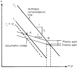
Based on the literature [22] and according to Fig. 2, the improved hardening parameter for considering time effect is as follows:

11

p_{c} = p_{c} (ε_{v}^{p}, t_{v}) .

Considering the time factor, Fig. 2 can be used to derive a void ratio increment as follows:

12

- Δ e = ψ l n (1 + \frac{Δ t_{v}}{t_{v}}) = (λ - κ) l n (1 + \frac{Δ p_{c}}{p_{c}}) .

Eq. (12) can be reduced to:

13

\frac{Δ p_{c}}{p_{c}} = {(1 + \frac{Δ t_{v}}{t_{v}})}^{\frac{ψ}{λ - κ}} - 1 .

Fig. 1Schematic view of the yield surfaces in q-p stress space

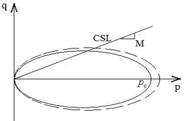
Fig. 2Incorporation of time factor in isotropic consolidation and rebound test parameters

Taking the Taylor series expansion for Eq. (13), it obtains:

14

\frac{\partial p_{c}}{\partial t_{v}} = \frac{ψ}{λ - κ} \frac{p_{c}}{t_{v}} .

Applying the total differential definition for Eq. (14) and combining Eqs. (10) and (14), it can derive the following:

15

d p_{c} = {\frac{\partial p_{c}}{\partial ε_{v}^{p}}|}_{t_{v}} d ε_{v}^{p} + {\frac{\partial p_{c}}{\partial t_{v}}|}_{ε_{v}^{p}} d t_{v} = \frac{1 + e}{λ - κ} p_{c} d ε_{v}^{p} + \frac{ψ}{λ - κ} \frac{p_{c}}{t_{v}} d t .

2.2.3. Flow rule

According to the theory of plasticity, plastic deformation $d ε_{i j}^{p}$ is divided into plastic volume strain $d ε_{v}^{p}$ and deviatoric strain $d e_{i j}^{p}$ :

16

d ε_{v}^{p} = Λ \frac{\partial F}{\partial \bar{p}} = Λ \frac{4}{3} M^{2} (\bar{p} - \frac{1}{2} p_{c}),

17

d e_{i j}^{p} = Λ \frac{\partial F}{\partial {\bar{s}}_{i j}} = Λ 2 {\bar{s}}_{i j},

where:

Λ = \frac{1}{{\bar{K}}_{p}} [\frac{\partial F}{\partial {\bar{σ}}_{_{k l}}} d {\bar{σ}}_{_{k l}}] = \frac{1}{K_{p}} [\frac{\partial F}{\partial {\bar{σ}}_{_{k l}}} d σ_{k l}],

and ${\bar{K}}_{p}$ is the point of reference for the bounding surface plastic modulus; and $K_{p}$ is the current stress point of the plastic modulus. Two of these plastic modulus values use the recommendation of Manzaei [23], as shown below:

18

K_{p} = {\bar{K}}_{p} + H_{0} \frac{16 M^{4} ν}{9 (λ - κ)} {\bar{p}}^{3} （\frac{b - 1}{b}） = \frac{8 M^{4} ν}{9 (λ - κ)} p_{c} (\bar{p} - \frac{p_{c}}{2}) \bar{p} + H_{0} \frac{16 M^{4} ν}{9 (λ - κ)} {\bar{p}}^{3} （\frac{b - 1}{b}） .

2.3. The elastic part

The function is:

19

d ε_{v}^{e} = \frac{d p}{K}, d e_{i j}^{p} = \frac{d s_{i j}}{2 G},

where $d ε_{v}^{e}$ is the elastic volumetric strain increment, and according to Hooke’s law:

K = \frac{ν p}{κ}, G = \frac{3 K (1 - 2 μ)}{2 (1 + μ)} .

2.4. Implicit integration of the model

Based on the concept of the implicit backward Euler method [24], calculation steps can be divided into two steps: (1) the elastic response and (2) viscoplastic correction. According to Eq. (1)-(19) and ref. [25], the derivation formulas can be obtained, as detailed in the appendix A.

The Newton-Raphson algorithm was used to solve the equation sets ( $R_{i}$ ) also in the appendix A [26]. The iterations were stopped when the iterative error $R_{i}^{(k)}$ was less than the allowable values. When $k$ iteration is used to calculate $\partial R_{i}^{(k)} / \partial (X)_{n + 1}$ and $\partial R_{i}^{(k)} / \partial (X)_{n + 1} \cdot δ (X)_{n + 1} = - R_{i}$ , then the tangent modulus is obtained at the same time (see appendix A).

3. The parameters of model

The time-dependent bounding surface model combines the advantages of the Mesri creep model, critical state soil mechanics theory, and the boundary surface model theory [27]. Meanwhile, the parameters are concise and easy to determine. This work focuses on the study of soft soil, and the following parameter influence analysis can be obtained via laboratory test data.

3.1. Creep parameters

Given Eq. (4), it can obtain a linear relation between $1 / E_{d}$ and $ε_{d}$ , thereby obtaining parameters $a$ and $b$ . It then derived $E_{d} / S_{u}$ and $R_{f}$ [28, 29]. $S_{u}$ was obtained using indoor unconfined compressive strength tests. As shown in Fig. 3, the $σ_{d} ~ ε_{d}$ hyperbolic equation has been converted into a linear equation. This was calculated using the least square method results in the linear intercept $a$ and slope $b$ . The $E_{d} / S_{u}$ were obtained using $a$ and $S_{u}$ . The analysis parameters under the condition of differing dynamic amplitudes are shown in Fig. 4.

Analysis parameters ( $R_{f}$ ) under the condition of different dynamic amplitudes are shown in Fig. 5. Using Eq. (9) to calculate the parameter $m$ from dynamic strain vs. time relationship curve in Fig. 6.

Fig. 31/Ed~εd relationship diagram

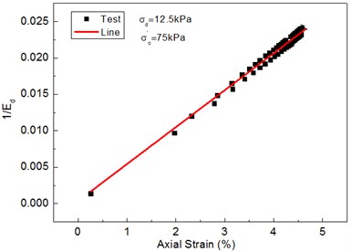
Fig. 4Ed/Su~Fd relationship diagram

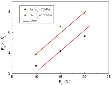
Fig. 5Rf~Fd relationship diagram

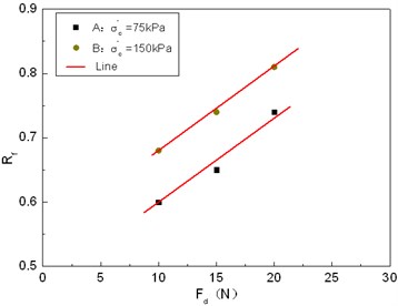
Fig. 6Strain vs. time relationship diagram

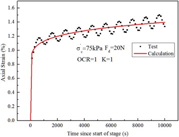
Fig. 7The q~p relationship in consolidated drained conditions

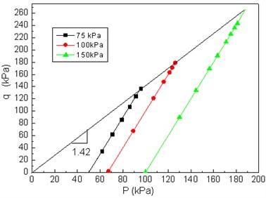
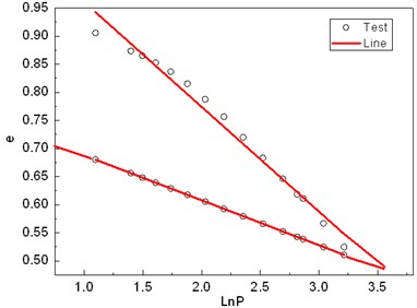
Fig. 8The isotropic consolidation and rebound test

3.2. Critical state model parameters

Based on critical state soil mechanics theory, the critical stress ratio $M$ in Fig. 7 can be obtained through the consolidated drained test; $q$ represents the effective deviatoric stress; $p$ is the effective confining pressure. The isotropic consolidation and rebound experiments were used to obtain the parameters $λ$ and $κ$ .

3.3. Plastic modulus parameter $H_{0}$

Parameter $H_{0}$ affects the form’s $q ~ ε$ relation curve, and the numerical size can determine a hardening or softening curve, as shown in Fig. 9.

Fig. 9Diagram of H0 effect on the q~ε relationship

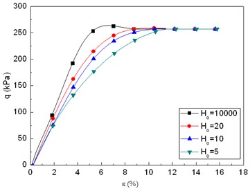
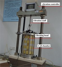
Fig. 10GDS dynamic triaxial apparatus

4. Experimental study and verification analysis

4.1. Dynamic experimental study

Shield segment and the structure can be affected by moving metro dynamic loads during vibration operation [30, 31]. Studies have shown that the metro dynamic loads produce a vibration waveform that is similar to the sine wave [32]. We performed a GDS dynamic triaxial test on soft soil. As illustrated in Fig. 10, during operation, the vibration staff (controlled by the vibration controller) drives the vibration head oscillating up and down so that vibration loading is applied to the soil in the cell chamber. The location of the soil is in Hexi area of Nanjing, China, Metro line 2 of Nanjing crosses through the area, and the physical and mechanical indexes of soft soil are shown in Table 1 [33].

The samples were prepared as the cylinders that were 38 mm in diameter and 75 mm in height. The effective confining pressure is, respectively, 75 and 150 kPa. We used a half sine wave load; dynamic amplitudes of 10, 15, and 20 N, respectively; and established 10000 vibration times.

Table 1Physical and mechanical properties of soft clay

$w$ (%)	$G_{s}$	$I_{p}$	$ρ$ (g/cm³)	$e_{0}$
37.3	2.72	17	1.877	0.99

4.2. Comparison and analysis

We selected the confining pressure of $σ_{d} =$ 75 kPa, a dynamic amplitude of $F_{d} =$ 10 N, and a vibration frequency $f =$ 1 Hz as an example. We then compared calculations results with the test results. The test parameters are as show in Table 2.

Table 2Parameters of model for clay

$E_{d} / S_{u}$	$R_{f}$	$m$	$C_{α}$	$M$	$λ$	$κ$	$H_{0}$
3.5	0.72	0.17	0.091	1.42	0.18	0.08	20

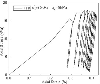
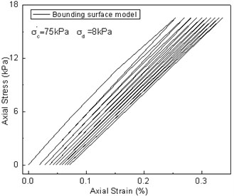
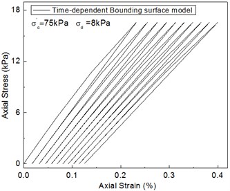
As shown in Fig. 11, the test results are compared against the calculation results of the $q ~ ε_{d}$ curve. The calculated results by the time-dependent bounding surface model are closer to the experimental value.

As shown in Fig. 12, the calculated results by the time-dependent bounding surface model are closer to the experimental value when compared with the result of strain vs. time curve.

Fig. 11Comparison between test results and predicted values of the q~εd curve

a)

b)

c)

Fig. 12Comparison between test results and predicted values of the strain vs. time curve

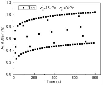
a)

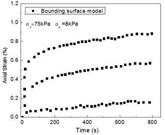
b)

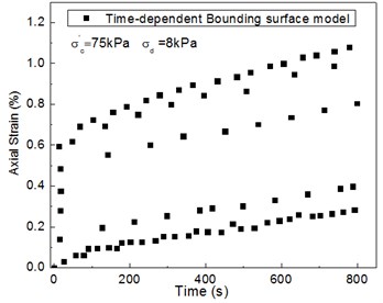
c)

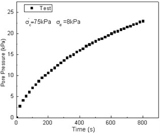
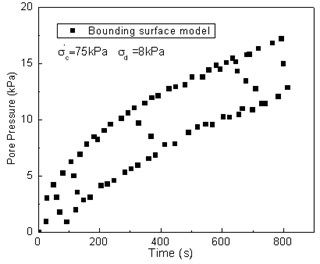
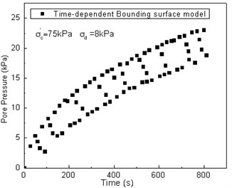
As shown in Fig. 13, the calculated results by the bounding surface model are small when compared with the result of the pore pressure vs. time curve, and the calculated results enter a stable state. The calculated results by the time-dependent bounding surface model is similar to the measured data. Although the turning point is small, it is consistent with the test value as they both increase over time.

Via the above curve comparisons between test results and prediction, we can see that the time-dependent bounding surface model could effectively describe the dynamic characteristics of soft soil under dynamic loads.

Fig. 13Comparison between test results and predicted values of the pore pressure vs. time curve

a)

b)

c)

5. Conclusion

This paper studies the dynamic characteristics of soft soil under metro dynamic loads. The conclusions can be drawn from this study:

1. Introducing the Mesri creep model into the boundary surface model allows for the calculation of soil creep under arbitrarily shear stress levels; the shear stress level contains all the stress level statuses (0-100 %). The improved bounding surface model can take into consideration the time effects.

2. The calculation steps have been provided to illustrate the time-dependent bounding surface model using the Newton-Raphson method and carried out secondary development of model.

3. Simulating the dynamic load waveforms had been carried out during GDS dynamic triaxial test for the soft soil, comparing the test results with predicted values. The results showed that the time-dependent bounding surface model more accurately calculated the dynamic strain.

References

Bjerrum L. Engineering geology of Norwegian normally consolidated marine clays as related to settlements of buildings. 7th Rankine Lecture. Geotechnique, Vol. 17, Issue 2, 1967, p. 83-117.

Search CrossRef
Luo J. H., Miao L. C., Wang Z. X., et al. Modified cam-clay model with dynamic shear modulus under cyclic loads. Journal of Vibroengineering, Vol. 17, 2015, p. 112-124.

Search CrossRef
Zhang J. F., Chen J. J., Wang J. H. Prediction of tunnel displacement induced by adjacent excavation in soft soil. Tunneling and Underground Space Technology, Vol. 36, 2013, p. 24-33.

Search CrossRef
Dafalias Y. F., Popov E. P. A model of non-linearly hardening materials for complex loading. Acta Mechanica, Vol. 21, 1975, p. 173-192.

Search CrossRef
Dafalias Y. F., Herrmann L. R. Bounding surface plasticity. I: Mathematical foundation and hypo-plasticity. Journal of Engineering Mechanics, Vol. 112, Issue 9, 1986, p. 966-987.

Search CrossRef
Dafalias Y. F., Herrmann L. R. Bounding surface plasticity. II: Application to isotropic cohesive soils. Journal of Engineering Mechanics, Vol. 112, Issue 12, 1986, p. 1292-1318.

Search CrossRef
Wood D. M. Soil Behavior and Critical Soil Mechanics. Cambridge University Press, 1990.

Search CrossRef
He Z. J., Zhang J. X. Strength characteristics and failure criterion of plain recycled aggregate concrete under triaxial stress states. Construction and Building Materials, Vol. 54, 2014, p. 354-362.

Search CrossRef
Hu C., Liu H. X., Huang W. Anisotropic bounding-surface plasticity model for the cyclic shakedown and degradation of saturated clay. Computers and Geotechnics, Vol. 44, 2012, p. 34-47.

Search CrossRef
Wang Gang, Zhang Jian-Min Implementation and application of a bounding surface model in MARC. Rock and Soil Mechanics, Vol. 27, Issue 9, 2006, p. 1535-1540, (in Chinese).

Search CrossRef
Singh A., Mitchell J. K. General stress-strain-time function for soils. Journal of Soil Mechanics and Found Engineering Division, American Society of Civil Engineering, Vol. 94, Issue 1, 1968, p. 21-46.

Search CrossRef
Kondner R. L. Hyperbolic stress-strain response: cohesive soils. Journal of Soil Mechanics and Foundations, American Society of Civil Engineering, Vol. 89, Issue 1, 1963, p. 115-143.

Search CrossRef
Mesri G., Febres C. E., Shields D. R., Castro A. Shear-stress-strain-time behavior of clays. Geotechnique, Vol. 31, Issue 4, 1981, p. 537-552.

Search CrossRef
Shalabi F. I. FE analysis of time-dependent behavior of tunneling in squeezing ground using two different creep models. Tunneling and Underground Space Technology, Vol. 20, 2005, p. 271-279.

Search CrossRef
Feng S. Y., Wei L. M., He C. Y., He Q. A computational method for post-construction settlement of high-speed railway bridge pile foundation considering soil creep effect. Journal of Central South University of Technology, Vol. 21, 2014, p. 2921-2927.

Search CrossRef
Victor N. K. Parameter estimation for time-dependent bounding surface models for cohesive soils. Soil Constitutive Models, 2005, p. 237-256.

Search CrossRef
Bodas Freitas T. M., David M. P., Lidija Z. A time dependent constitutive model for soils with isotach viscosity. Computers and Geotechnics, Vol. 38, 2011, p. 809-820.

Search CrossRef
Hardin B. O., Black W. L. Vibration modulus of normally consolidated clay. Journal of the Soil Mechanics and Foundations Division, Vol. 94, Issue 2, 1968, p. 353-369.

Search CrossRef
Hardin B. O., Drnevich V. P. Shear modulus and damping in soils: design equations and curves. Journal of the Soil Mechanics and Foundations Division, Vol. 98, Issue 7, 1972, p. 667-692.

Search CrossRef
Taylor D. W. Fundamentals of Soil Mechanics. Wiley. Literary Licensing, LLC, New York, 1948.

Search CrossRef
Papon A., Yin Z.-Y., Riou Y. Time homogenization for clays subjected to large numbers of cycles. International Journal for Numerical and Analytical Methods in Geomechanics, Vol. 37, Issue 11, 2013, p. 1470-1491.

Search CrossRef
Borja R. I., Kavazanjian J. R. E. A constitutive model for the stress-strain-time behavior of ‘wet’ clays. Geotechnique, Vol. 35, Issue 3, 1985, p. 283-298.

Search CrossRef
Manzari M. T., Nourm A. On implicit integration of bounding surface plasticity models. Computers and Structures, Vol. 63, Issue 3, 1997, p. 385-395.

Search CrossRef
Xu T. H., Zhang L. M. Numerical implementation of a bounding surface plasticity model for sand under high strain-rate loadings in LS-DYNA. Computers and Geotechnics, Vol. 66, 2015, p. 203-218.

Search CrossRef
Manzari M. T., Prachathananukit R. On integration of cyclic soil plasticity model. Numerical and Analytical Methods in Geomechanics, Vol. 25, Issue 6, 2001, p. 525-549.

Search CrossRef
Amorosi A., Boldini D., Germano V. Implicit integration of a mixed isotropic-kinematic hardening plasticity model for structured clays. International Journal for Numerical and Analytical Methods in Geomechanics, Vol. 32, Issue 10, 2008, p. 1173-1203.

Search CrossRef
Mašín D. Hypoplastic cam-clay model. Geotechnique, Vol. 62, Issue 6, 2012, p. 549-553.

Search CrossRef
Subramaniam P., Sunbhadeep Banerjee Shear modulus degradation model for cohesive soils. Soil Dynamics and Earthquake Engineering, Vol. 53, 2013, p. 210-216.

Search CrossRef
Jun Wang, Yuan qiang Cai, Fang Yang Effects of initial shear stress on cyclic behavior of saturated soft clay. Marine Georesources and Geotechnology, Vol. 31, Issue 1, 2013, p. 86-106.

Search CrossRef
Shen Shui-Long, Wu Huai-Na, Cui Yu-Jun Long-term settlement behaviour of metro tunnels in the soft deposits of Shanghai. Tunneling and Underground Space Technology, Vol. 40, 2014, p. 309-323.

Search CrossRef
Ng C. W. W., Liu G. B., Li Q. Investigation of the long-term tunnel settlement mechanisms of the first metro line in Shanghai. Canadian Geotechnical Journal, Vol. 50, Issue 6, 2013, p. 674-684.

Search CrossRef
Zhang Jun-Feng, Chen Jin-Jian, Wang Jian-Hua Prediction of tunnel displacement induced by adjacent excavation in soft soil. Tunneling and Underground Space Technology, Vol. 36, 2013, p. 24-33.

Search CrossRef
Alpan I. The geotechnical properties of soils. Earth-Science Reviews, Vol. 6, Issue 1, 1970, p. 5-49.

Search CrossRef

About this article

Received

26 August 2015

Accepted

12 November 2015

Published

30 December 2015

SUBJECTS

Vibration in transportation engineering

Keywords

metro dynamic loads

dynamic characteristics

vibration

soft clay

time-dependent

Acknowledgements

The authors gratefully acknowledge the financial support for this research from the National Natural Science Foundation of China (Grant Nos. 51278099, 51578147) and the Postgraduate Research and Innovation Plan Project in Jiangsu Province (Grant No. CXLX13_098). We thank LetPub (www.letpub.com) for its linguistic assistance during the preparation of this manuscript.

This is an open access article distributed under the Creative Commons Attribution License, which permits unrestricted use, distribution, and reproduction in any medium, provided the original work is properly cited.