The application of peridynamics in predicting beam vibration and impact damage

1. Introduction

The peridynamic (PD) theory was first proposed by Silling [1] as a nonlocal theory for modeling the deformation of solid materials subjected to mechanical loading. A central characteristic of peridynamic models is an absence of spatial derivatives of the displacement field. This theory assumes that particles in a continuum interact with each other across a finite distance, as in molecular dynamics. It reformulates the basic equations of motion in such a form that the internal forces are evaluated through an integral formulation that does not require the evaluation of a stress tensor field or its spatial derivatives [2]. Damage is incorporated in the theory at the level of these two particle interactions, so localization and fracture occur as a natural outgrowth of the equation of motion and constitutive models [3]. In additional to solid mechanics, peridynamic theory has been extended to model composite materials, fluids, heat transfer and explosives [4, 5].

The majority of the work on peridynamic theory to date has focused on damage prediction in many problems in solid mechanics. However, there has been little work investigating vibration analysis for structural mechanics (beams, plates and shells). Therefore, this paper presents the new numerical method for beam vibration analysis and impact damage using peridynamic theory. In Classical Continuum Mechanics we normally use 1D Euler-Bernoulli beam theory which is a fourth partial derivative of displacement to study the beam transverse vibration. For peridynamic theory, although the 1D peridynamic model is simple and calculation saved, it can’t be used directly to calculate the beam transverse vibration as the 1D model can’t resist bending. Recently some novel 1D peridynamic models are developed to solve the difficulty in modeling Euler-Bernoulli beam. In order to predicting the deformation of Timoshenko beam using one-dimensional beam structure, a new bond based peridynamic model is derived involving the equilibrium equations for transverse force and bending moment [6]. Considering additional micro-rotational degrees of freedom to each material node, a 1D state-based micropolar peridynamic model is proposed to predict the beam transverse vibration and scale stiffening response of beams [7]. Similarly, from the concept of a rotational spring between bonds, a new 1D state-based peridynamic material model is presented that could directly resist bending deformation, and successfully reproduces accurate deformation results for a simple beam [8].

Obviously the framework of these developed 1D models has to be rewritten as well as the corresponding computation program. However, the 2D peridynamic model of the beam could capture resistance to bending naturally as the transverse displacement is contained in the model. If the 2D peridynamics is applied, the model could be used for the structural vibration and crack propagation analysis directly and don’t need to be modified anymore. In the presented study we provides a complete solution for the deformation and impact damage of elastic peridynamic beams. We discuss the convergence of peridynamic solution to that of the classical, local, elasticity solution. Several typical cases is carried out for the comparison.

The paper is organized as follows: Firstly, we briefly review the peridynamic theory. In Section 2, we state the fundamental integro-differential equation of peridynamic theory and relevant parameters. After introducing the basic framework of peridynamic theory, numerical techniques adopted for the simulations are briefly explained. In Section 3, we apply peridynamics to solve the vibration response of beams. We first discuss the simulation of free vibration of a simple supported beam and verify the numerical methods when trying to compare the peridynamic solutions with those of classical elasticity. In the following examples, we demonstrate the ability of peridynamics to model deformation of an axially moving system. To further demonstrate the capabilities of the model, the failure process of three-point bending beam with offset notch is studied. Finally, Section 4 contains a summary and conclusions of this work.

2. Peridynamic theory

In the peridynamic theory, a continuous body is considered to consist of material points that interact in a nonlocal manner. In other words, a material point interacts with all other material points within some neighborhood of the point. The assumption is made that Newton’s second law of motion is valid at each material point. The state of any material point is determined by its pairwise interaction with the points that are located within a finite distance, called the horizon, which is symbolized by $\delta$. Any pair of material points only interact with each other when the distance between them is less than the horizon. The peridynamic equation of motion for any material point at position $x$ and time $t$ can be expressed by:

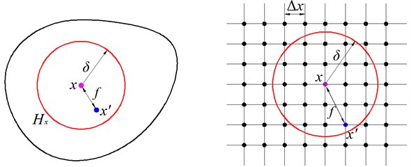
where $H_x$ is a spherical neighborhood of given radius $\delta$ centered at point $x$ in the reference configuration, $\rho$ is mass density, $u$ is displacement vector, $b$ is prescribed body force vector density, and $f$ is the pairwise force exerted on particle $x$ in the peridynamic bond that connects particle $x$ to $x\text{'}$. The nonlocal interaction of material points via the force function is illustrated in Fig. 1.

Eq. (1) is the fundamental integro-differential equation of peridynamic theory. It is based on Newton’s second law for all points within the domain of analysis and does not contain any spatial derivatives. All constitutive properties of a material in PD method are given by specifying the vector-valued pairwise force function, $f$. Silling [1] proposed that the pairwise force function, $f$, depends on the relative position, $\xi =x\text{'}-x$, of the two interacting points and their relative displacement, $\eta =u\text{'}-u$, thus leading to the functional form of $f=f(\xi ,\eta )$. Silling and Askari [3] defined a form of pairwise function for isotropic material as:

in which $\xi$ is the relative position and $\eta$ is the relative displacement, accordingly, $\xi +\eta$ represents the current relative position vector between the two particles, $c$ is material property in peridynamics, and $s$ is bond stretch, defined by:

where $s$ is positive when the bond is in tension and negative when the bond is in compression.

Fig. 1Interaction of a material point with its neighboring points and numerical grid for evaluating

The material property $c$ is determined by equating the peridynamic internal energy of a body to the strain energy density from the classical elasticity theory. For 2D peridynamics concerned here, it can be found to be:

where $E$ is the elastic Young’s modulus and the Poisson’s ratio is set as $\nu =$ 1/3.

Damage of a peridynamic material at point $x$ can be defined locally in term of the ratio of amount of broken bonds to total amount of interactions [1, 3] as:

where $\mu (x,\xi ,t)$ is a factor mapping the breakage of bond:

and $s_0$ is the critical stretch for bond failure in the material, which can be correlated with the energy release rate quantity in the classical theory [12]:

where $G_0$ represents the critical energy release rate.

In the peridynamic theory, fracture occurs naturally in a PD body as a consequence of the equation of motion and the constitutive model. Fractures initiate, grow, turn, branch, and arrest without the need for any externally supplied law or special techniques to control these processes, as is required in traditional models for fracture mechanics. Material defects can evolve in any modes not known in advance allows the PD approach to model complex patterns of mutually interacting cracks within a body.

Numerical solutions are needed for most peridynamic analyses. In order to carry out the numerical integration, the region of interest is first discretized into uniform regular subdomains in which the displacement and velocity fields are assumed to be constant. Hence, each sub-domain can be represented as a single collocation point located at the mass center of the subdomain. All the governing equations are then rewritten for these points along with a Riemann-sum type approximation over each horizon for the integro-differential equation (Eq. (1)). This discretization results in a set of algebraic equations with displacement at the different points as unknowns, which are solved for after proper imposition of boundary conditions. During the discretizing process, we should pay special attention on the surface effect in peridynamic method. The pairwise function given in Eq. (2) is derived under the assumption that the material point located at $x$ is in a single material with its complete neighborhood entirely embedded within its horizon $\delta$. However, this assumption becomes invalid when the material point is close to free surfaces where the horizon extends outside the physical domain. If one simply assumes the micro-elastic modulus drops to zero outside of the physical domain, there will be an unreasonable reduction in material stiffness near the free surfaces which will causes the numerical results deviate from Classical Continuum Mechanics (CCM). This is called peridynamic “surface effect” [9]. Since free surfaces vary from one problem to another, it is impractical to resolve this issue analytically. Therefore, the stiffness inaccuracies due to free surfaces is revised numerically by a parameter termed surface correction factor $G$, as explained in literature [10]. Considering the surface effects, the discrete form of the equations of motion given in Eq. (1) can be written as:

where superscript $n$ is the time step number, $i$ represents the point in question, and $j$ represents the point within the horizon of $i$, $G_{ij}$ is the correction factor for a peridynamic bond between material points $x_i$ and $x_j$, $V_j$ is the volume of node $j$ and is represented by square lattice area in 2D model that describes a portion of the body assigned to a point.

To solve the second derivative ordinary differential equations (Eq. (5)), an explicit time integration method, i.e. Velocity-Verlet algorithm [11], which is more numerically stable than central-differences, is used for the peridynamic analysis:

where $u$, $\dot{u}$ and $\ddot{u}$ are displacement, velocity, and acceleration vectors, respectively.

3. Numerical illustrations

3.1. Free vibration of a simple supported beam

In order to demonstrate the validity of the 2D peridynamic model, especially the effect of surface correction factors (SCF) on the dynamic response of beam vibration, we carry out a simple test case first: a simply supported beam. The geometric and material properties considered for the beam model are: $L=$ 0.1 m, $h=$ 0.005 m, $b=$ 0.005 m, $E=$ 71 GPa, $\rho =$ 2700 kg/m³, where $L$, $h$ and $b$ are length, thickness and width of the beam respectively, as shown in Fig. 2. Here, low thickness to length ratio of the beam allows the Euler-Bernoulli type model to be applicable in the case. Please note that while these parameters may not be physically representative, they are adequate for the purpose of demonstration of peridynamic validity. It is convenient to calculate the first order free vibration period of the beam as $T=2L^2/\pi /h\bullet {\left(12\rho /E\right)}^{0.5}=$0.86 ms according to Euler-Bernoulli beam theory.

Fig. 2Schematic of a simple supported beam

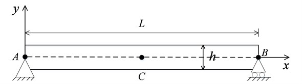
To implement the simply-supported condition in peridynamics, it is sufficient to constrain the displacement of a single point for each support, i.e. node $A$ and node $B$ as shown in Fig. 2:

12

$u_x^A=u_y^A=0,$

13

$u_y^B=0.$

The beam undergoes free bending vibrations of small amplitude about the $x$-axis such that the deflection is consistent with the linear Euler-Bernoulli theory. That is, any plane cross-section initially perpendicular to the axis of the beam remains plane and perpendicular to the neutral surface during bending. Thus, the relationship between longitudinal displacement $u_x(x,y,t)$ and transversal displacement $u_y(x,y,t)$ is given by:

14

$u_x\left(x,y,t\right)=-y\frac{\partial u_y\left(x,y,t\right)}{\partial x}.$

Accordingly, the initial deflection of the simple supported beam is set as:

15

$u_x\left(x,y,0\right)=-yU\frac{\pi }{L}\mathrm{c}\mathrm{o}\mathrm{s}\left(\frac{\pi }{L}x\right),\mathrm{}$

16

$u_y\left(x,y,0\right)=U\mathrm{s}\mathrm{i}\mathrm{n}\left(\frac{\pi }{L}x\right),$

where the amplitude is chosen as $U=$ 3×10^-3 mm.

3.1.1. Numerical convergence in peridynamics

In peridynamics the value of horizon $\delta$ is chosen according to the physical characteristics of the object to be modeled. For the problem of bending in a thin plate or beam, the thru-thickness discretization plays a significant role in properly capturing resistance to bending. Thus, the horizon size needs to be selected sufficiently small relative to the thickness of the beam so that bending is not influenced by the size of the nonlocal region at a point. Meanwhile, it is proposed in practice that the appropriate value of grid spacing $\mathrm{\Delta }x$ is chosen proportionate to the peridynamic horizon, i.e. $\delta =\left(3\text{-}4\right)\mathrm{\Delta }x$, as a balance between accuracy and computational efficiency for a particular horizon [3, 12]. In order to get the proper peridynamic discretization parameters, it is essential to study the convergence of peridynamic solution, such as beam vibration period, to the analytical solution. The calculation is carried out with all parameters held constant, but six different values of horizon, $\delta =$ 5 mm, 2.5 mm, 2 mm, 1.5 mm, 1.25 mm, and 1 mm with grid spacing $\mathrm{\Delta }x\approx \text{1/4}\delta$. Table 1 shows the beam vibration periods and corresponding relative errors to analytical solution based on different horizon values. As expected, the peridynamic solution becomes closer to the analytical solution if the horizon $\delta$ decreases. This means that sufficient discretizing horizon number in thickness direction is necessary for the bending analysis of a long, slender beam structure. It seems to be ideal to use small $\delta$ in peridynamic analysis. However, this will pose a significant increase in computational time. Consequently, $\delta =$ 1 mm and $\mathrm{\Delta }x=$ 0.25 mm will be used in subsequent numerical investigations.

Table 1Convergence for vibration period for the simple supported beam example. Relative errors from the classical analytical solution

Horizon size, $\delta$ / mm	Grid spacing, $\mathrm{\Delta }x$ / mm	Number of horizon in thickness	Vibration period, ms	Relative error (%)
5.0	1.2	1.0	0.98	14
2.5	0.6	2.0	0.90	4.7
2.0	0.5	2.5	0.875	1.7
1.5	0.35	3.3	0.87	1.2
1.25	0.3	4.0	0.88	2.3
1	0.25	5.0	0.865	0.6

3.1.2. Effect of surface correction factors

The transverse displacement of the midpoint (point $C$ in Fig. 2) is shown in Fig. 3. In order to investigate the effect of surface correction factor on PD solution, the calculation without surface correction factor is also shown in Fig. 3. For comparison, exact solution considering the Euler-Bernoulli model is reported simultaneously in Fig. 3. It is obvious that considering surface correction factor the peridynamic solution is almost identical to that of classic continuum mechanics. However, the result without considering surface correction factor shows the “soft boundary effect” which leads to a longer vibration period of the beam. In 1D peridynamics, the problem of softening boundary could be solved by extending a hypothesized domain outside each support of the beam [6]. However, the approach cannot be used in the 2D peridynamic model for a slender beam transverse vibration. The reason is that outstretching the beam outside the supports just modify the stiffness in axial direction. If the same technique is applied in beam thickness direction, the beam vibration characteristics will be changed greatly due to the thickness sensitivity of the structure. Therefore, surface correction factor is an indispensable and reliable method to eliminate the “surface effect” in peridynamics. In the following calculations, the surface correction factor is applied in the peridynamic models.

Fig. 3Beam midpoint transverse displacement response

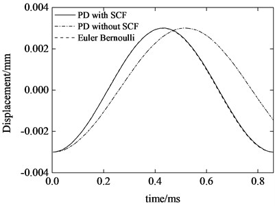
Fig. 4Beam midpoint transverse velocity response

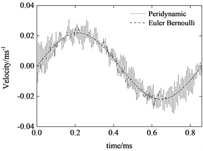
Fig. 4 is the transverse vibration velocity of midpoint $C$. We can see that the velocity curve of peridynamics shows high frequency content which is different from that of Euler-Bernoulli result. The reason is that the material points in the domain not only proceed the “macroscopical” movement, but also vibrate around their “equilibrium” position.

3.2. Dynamic response of an axially moving beam

In order to further investigate the ability of the 2D peridynamics proposed above for predicting more complicated beam vibration behavior, the bending of an axially moving cantilever beam is taken into consideration. Consider the axially moving cantilever beam with the following parameters: $L_0=$0.1 m, $h=$ 0.005 m, $b=$ 0.005 m, $E=$ 71 GPa, $\rho =$ 2700 kg/m³, $v_0=$10 m/s, where $L_0$, $h$ and $b$ are initial outstretched length, thickness and width of the beam respectively, $v_0$ is beam axially moving speed, as shown in Fig. 5.

Fig. 5Schematic of an axially moving cantilever beam with a constant speed v0

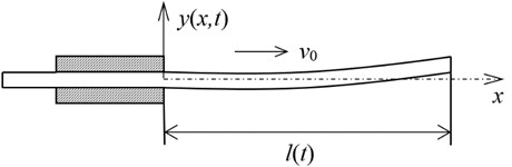
In order to achieve clamped boundary conditions, the displacements in y direction are set to zero in boundary region. The beam proceeds with free vibration under the following initial deformation which is in proportion to the first vibration mode of cantilever beam under initial outstretched length:

17

$u_x\left(x,y,0\right)=-U{\mathrm{\lambda }}_{1}y\left(\mathrm{s}\mathrm{h}{\mathrm{\lambda }}_{1}x+\mathrm{s}\mathrm{i}\mathrm{n}{\mathrm{\lambda }}_{1}x-\frac{\mathrm{s}\mathrm{h}{\mathrm{\lambda }}_1{L}_0-\mathrm{s}\mathrm{i}\mathrm{n}{\mathrm{\lambda }}_1{L}_0}{\mathrm{c}\mathrm{h}{\mathrm{\lambda }}_1{L}_0+\mathrm{c}\mathrm{o}\mathrm{s}{\mathrm{\lambda }}_1{L}_0}\left(\mathrm{c}\mathrm{h}{\mathrm{\lambda }}_{1}x-\mathrm{c}\mathrm{o}\mathrm{s}{\mathrm{\lambda }}_{1}x\right)\right),$

18

$u_y\left(x,y,0\right)=U\left(\mathrm{c}\mathrm{h}{\mathrm{\lambda }}_{1}x-\mathrm{c}\mathrm{o}\mathrm{s}{\mathrm{\lambda }}_{1}x-\frac{\mathrm{s}\mathrm{h}{\mathrm{\lambda }}_1{L}_0-\mathrm{s}\mathrm{i}\mathrm{n}{\mathrm{\lambda }}_1{L}_0}{\mathrm{c}\mathrm{h}{\mathrm{\lambda }}_1{L}_0+\mathrm{c}\mathrm{o}\mathrm{s}{\mathrm{\lambda }}_1{L}_0}\left(\mathrm{s}\mathrm{h}{\mathrm{\lambda }}_{1}x-\mathrm{s}\mathrm{i}\mathrm{n}{\mathrm{\lambda }}_{1}x\right)\right),$

where ${\lambda }_1$ is the first root of transcendental equation $1+\mathrm{c}\mathrm{h}\left(\lambda L_0\right)\mathrm{c}\mathrm{o}\mathrm{s}\left(\lambda L_0\right)=$ 0, the initial amplitude is chosen as $U=$ 3×10^-3 mm.

Fig. 6Tip transverse displacement of the axially moving cantilever beam

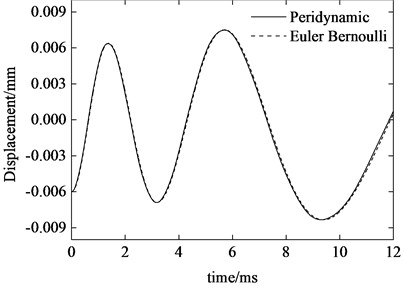
Fig. 7Tip transverse velocity of the axially moving cantilever beam

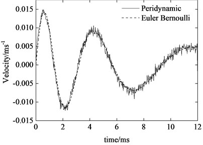
The two-dimensional peridynamic model is constructed by discretization of the beam with horizon $\delta =$ 1 mm and grid spacing $\mathrm{\Delta }x=$0.25. The time step size is 10^-8 s. Fig. 6 and 7 show the peridynamic solutions of the transverse displacement and velocity at right free end of the beam. For comparison, the solutions of Euler-Bernoulli model for the problem is also given in the figures. As can be seen, the peridynamic predictions are in excellent agreement with analytical solution. Similarly, the tip velocity curve of peridynamics also shows high frequency oscillations as numerically investigated in the case of simple supported beam. Furthermore, we can see that the vibration amplitude of displacement increases gradually while the velocity amplitude decreases. It is also noticeable that, during the ejection period, for the present case of axial motion, the vibration frequency rapidly diminishes as the length of the beam increases which is coincident with the conclusion in literature [13].

3.3. Dynamic crack propagation in a three-point bending beam with an offset notch

The three-point bending beam with an offset notch is extensively used to study the mixed I-II crack propagation in rock. In experiment, an offset notch was created in the specimen as preexisting crack tip. As a result of the applied load, the crack started propagating from the notch towards the top surface at an angle (clearly indicating the mixed mode fracture). In this section, the identical PD model is implemented to simulate the failure process in the experiment tested by John [14].

The geometric configuration of the experiment is given in Fig. 8. The PD simulations are performed by using 58 800 collocation points with a spacing of $\mathrm{\Delta }x=$ 0.5 mm. The horizon size is specified as $\delta =4\mathrm{\Delta }x$. The specimen is loaded by applying 60 MPa impact stress, ramped up over 1 μs and kept constant later, on the top edge shown in Fig. 8. In the simulations, a brittle material model is used for the specimen with elastic modulus of $E=$34.48 GPa, Poisson’s ratio of $\nu =$ 0.33 and critical stretch of $s_0=$0.00085. The peridynamic theory predicts the crack propagation behavior as shown in Fig. 9. The fracture initiates at the notch tips and begins to growth at the time of 90 μs. As it is observed in the experiment that the crack does not grow parallel to the notches. Instead, the crack path initially grows at about 30° to the notches and then curves towards but does not go to the point of application of load. At the time of 250 μs the crack runs through the whole specimen. As can be seen in Fig. 10, the peridynamic material model could predicts quite well the failure paths observed in the experiment.

Fig. 8Geometry of the three-point bending beam with offset notch (all dimensions in mm)

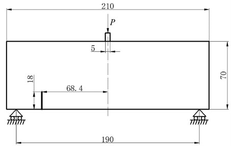
Fig. 9Damage maps (crack paths) for the three-point bending beam with an offset notch

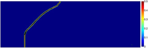
Fig. 10Comparison between numerical simulations and experimental results [14]

4. Conclusion

Peridynamics is a continuum theory based on a nonlocal force model. It’s has been successfully utilized for damage prediction in many problems. However, the peridynamic theory is seldom used in the structures vibration and mixed-mode fracture analysis. Therefore, this paper presents the application of peridynamic theory in predicting beams vibration and crack propagation process in a three-point bending beam. The surface correction factor is applied to solve the “softer” material near the boundary in peridynamics. It is found that with the surface correction factor the unreasonable reduction of material stiffness near the free surfaces of structures is successfully eliminated in the model. We have shown that, unlike 1D peridynamic model, the 2D model could accurately predict the vibration response of elastic beams without any modifying of the current theory framework. Furthermore, the 2D peridynamic theory could predict quite well the dynamic failure process in the three-point bending beam with an offset notch. It is found that the crack path initiates from the notch tip and growths with an angle from the notch direction until reaches the upper edge of the specimen.