Multi-layer neural network with deep belief network for gearbox fault diagnosis

1. Introduction

Gearboxes play crucial roles in the mechanical transmission systems, are used to transmit power between shafts and are expected to work 24 hours a day in the production system. Any failures with the gearboxes may introduce unwanted downtime, expensive repair and even human casualties. Therefore it is essential to detect and diagnose faults in the initial stage [1-4]. As an effective component for the condition-based maintenance, the fault diagnosis has gained much attention for the safe operations of the gearboxes. The gearbox conditions can be reflected by such measurements as vibratory, acoustic, thermal, electrical and oil-based signals [5-8]. Among above symptoms, the vibration analysis is the most commonly-used technique for the reason that every machine is considered to have a normal spectrum until there is a fault, where the spectrum changes [9, 10]. The vibration signals have been proven effective to reflect the healthy condition of the rotating machinery.

Various studies exist, of vibrations-based algorithms for detection and diagnostics of faults in gearboxes, among these are support vector machines and artificial neural network. A support vector machines based envelope spectrum was proposed by Guo et al. [11] to classify three health conditions of the planetary gearboxes. An intelligent diagnosis model based on wavelet support vector machine (SVM) and immune genetic algorithm (IGA) was proposed for the gearbox fault diagnosis [12]. The IGA was developed to determine the optimal parameters for the wavelet SVM with the highest accuracy and generalization ability. Tayarani-Bathaie et al. [13] suggested a dynamic neural network to diagnose the gas turbine fault. The artificial neural network combining with empirical mode decomposition was applied for automatic bearing fault diagnosis based on vibration signals [14]. Among all the typical classifiers, the support vector classification (SVC) family (i.e., the standard SVC and its variants) attracted much attention due to their extraordinary classification performance. According to the researches, the SVM family received good results in comparison with the peer classifiers.

Multi-layer neural networks, typically used in supervised learning to make a prediction or classification. As Y. Bengio in the literature [15, 16] reported, the gradient-based training of supervised multi-layer neural networks (starting from random initialization) gets easily stuck in “apparent local minima or plateaus”. That is to restrict its application for gearbox fault diagnosis. Since 2006, deep networks have been applied with success in classification tasks and other fields such as in regression, dimensionality reduction, and modeling textures [17], but few were used for the fault diagnosis cases. Tran et al. [18] introduced the application of the deep belief networks to diagnose reciprocating compressor valves. Tamilselvan and Wang [19] employed the deep belief learning based health state classification for iris dataset, wine dataset, Wisconsin breast cancer diagnosis dataset, and Escherichia coli dataset. The limited reports show the deep learning structure for the fault diagnosis with commonly one modality feature.

In this work, we combine deep learning strategies with multi-layer neural network for the identification and classification of gearbox faults, where complicated faults are considered that a fault signal usually includes one or several basic faults. The typical multi-layer neural network (MLNN) [20] is used firstly for the identification and classification of gearbox faults, where batch training strategy is used to train the neural network. Then several fine-tuning schemes for improving the typical multi-layer neural network by preventing co-adaptation of feature detectors are suggested for the gearbox faults identification and classification. At last, a MLNN-based deep learning technique is proposed, where the weights of neural network are initialized using deep belief network (DBN) [21].

To validate the robustness of the MLNN-based approaches, a fault condition pattern library is constructed, which has 58 kinds of combined fault patterns. 20 test cases are used and each test case has 12 kinds of condition pattern that are randomly selected from the pattern library. A large number of experiments show the multi-layer neural network with DBN (MLNN_DBN) has most excellent performance and achieves to avoid falling into “apparent local minima or plateaus”.

The rest of this paper is structured as follows. Section 2 introduces the used methodologies including multi-layer neural networks and proposed MLNN-based learning architecture using deep belief network; Section 3 introduces feature representations of vibratory signals. Section 4 presents the implementation of the classifier based on multi-layer neural network; Section 5 introduces experimental setup; results and discussion are presented in Section 6. Finally some conclusions are drawn.

2. Methodologies

In this section, multi-layer neural network is firstly introduced, and then several fine-tuning schemes are explained. At last, MLNN-based learning architecture using deep belief network (MLNN_DBN) is proposed for gearbox fault diagnosis.

2.1. Multi-layer neural network

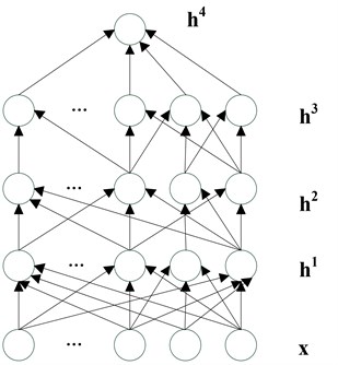
Multi-layer neural network is typically used in supervised learning to make a prediction or classification, through a series of layers, each of which combines an affine operation and a non-linearity. A typical set of equations for multi-layer neural network [17, 20] is the following. As illustrated in Fig. 1, layer $k$ computes an output vector ${\mathbf{h}}^k$ using the output ${\mathbf{h}}^{k-1}$ of the previous layer, starting with the input $\mathbf{x}=h^0$:

1

${\mathbf{h}}^k=\tanh \left({\mathbf{b}}^k+{\mathit{W}}^k{\mathbf{h}}^{k-1}\right),$

with parameters ${\mathbf{b}}^k$ (a vector of offsets) and ${\mathbf{W}}^k$ (a matrix of weights). The $\mathrm{t}\mathrm{a}\mathrm{n}\mathrm{h}(·)$ is can be replaced by $\mathrm{s}\mathrm{i}\mathrm{g}\mathrm{m}\left(\mathrm{u}\right)=1/\left(1+e^{-u}\right)=(\tanh \left(u\right)+1)/2$ or other saturating non-linearities [17]. The top layer output ${\mathbf{h}}^l$ is used for making a prediction and is combined with a supervised target $y$ into a loss function $L({\mathbf{h}}^l,y)$, typically convex in ${\mathbf{b}}^l+{\mathit{W}}^l{\mathbf{h}}^{l-1}$. The output layer might have a non-linearity different from the one used in other layers, e.g., the softmax:

2

${\mathbf{h}}_i^l=\frac{e^{b_i^l+W_i^l{\mathbf{h}}^{l-1}}}{\sum _j^{}{e}^{b_j^l+W_j^l{\mathbf{h}}^{l-1}}},$

where $W_i^l$ is the $i$th row of $W^l$, ${\mathbf{h}}_i^l$ is positive and ${\sum }_i{\mathbf{h}}_i^l=\text{1}$. The softmax output ${\mathbf{h}}_i^l$can be used as estimator of $P(Y=i|x)$, with the interpretation that $Y$ is the class associated with input pattern $\mathbf{x}$. In this case one often uses the negative conditional log-likelihood $\mathrm{L}\left({\mathbf{h}}^l,\mathrm{y}\right)=-\mathrm{l}\mathrm{o}\mathrm{g}P\left(Y=y|\mathbf{x}\right)=-\mathrm{l}\mathrm{o}\mathrm{g}{\mathbf{}\mathbf{h}}_y^l$ as a loss, whose expected value over ($\mathbf{x}$, $y$) pair is to be minimized [17]. The training of a MLNN is usually accomplished by using back propagation (BP) algorithm that involves two phases [20]:

– Forward phase: During this phase the free parameters of the network are fixed, and the input signal is propagated through the network of Fig. 1 layer by layer. The forward phase finishes with the computation of an error signal:

3

$e_i=d_i-y_i,$

where $d_i$ is the desired response and $y_i$ is the actual output produced by the network in response to the input ${\mathbf{x}}_i$.

– Backward phase: During this second phase, the error signal $e_i$ is propagated through the network of Fig. 1 in the backward direction. It is during this phase that adjustments are applied to the free parameters of the network so as to minimize the error $e_i$ in a statistical sense.

Fig. 1Multi-layer neural network

2.3. MLNN-based learning architecture using deep belief network (MLNN_DBN)

In this subsection, we propose a new fine-tuning strategy to improve the performance of typical MLNN. Training process of the proposed learning architecture includes two stages: A deep belief network is constructed firstly, and then is trained; after a certain amount of epochs, the weights of deep belief network are used to initialize the weights of the constructed MLNN; at last, the trained MLNN is used as classifiers to classify gearbox faults. The outline of MLNN-based learning architecture using deep belief network is as Fig. 2.

Fig. 2Outline of MLNN-based learning architecture using deep belief network

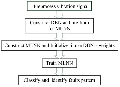
Fig. 3Deep belief network

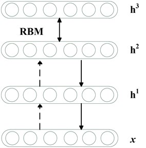
Deep belief networks (DBNs) [23] can be viewed as a composition of simple learning modules each of which is a restricted type of Boltzmann machine that contains a layer of visible units that represent the data and a layer of hidden units that learn to represent features that capture higher-order correlations in the data. It is a model in which the top two hidden layers form an undirected associative memory (see Fig. 3) and the remaining hidden layers form a directed acyclic graph that converts the representations in the associative memory into observable variables such as the pixels of an image. The two layers are connected by a matrix of symmetrically weighted connections, $\mathbf{W}$, and there are no connections within a layer. Given a vector of activities $v$ for the visible units, the hidden units are all conditionally independent so it is easy to sample a vector, $h$, from the factorial posterior distribution over hidden vectors, $p\left(\mathbf{h}\right|\mathbf{v},\mathrm{}\mathbf{W})$. It is also easy to sample from $p\left(\mathbf{v}\right|\mathbf{h},\mathrm{}\mathbf{W})$. By starting with an observed data vector on the visible units and alternating several times between sampling from $p\left(\mathbf{h}\right|\mathbf{v},\mathrm{}\mathbf{W})$ and $p\left(\mathbf{v}\right|\mathbf{h},\mathrm{}\mathbf{W})$, it is easy to get a learning signal. This signal is simply the difference between the pairwise correlations of the visible and hidden units at the beginning and end of the sampling.

The key idea of deep belief nets is that the weights, $\mathbf{W}$, learned by a restricted Boltzmann machine define both $p\left(\mathit{v}\right|\mathit{h},\mathit{W})$, and the prior distribution over hidden vectors, $p(\mathit{h},\mathit{W})$, so the probability of generating a visible vector, $v$, can be written as:

5

$p\left(v\right)=\sum _{h}p\left(h|W\right)p\left(v|h,W\right).$

The training algorithm for DBNs proceeds as follows. Let $\mathbf{X}$ be a matrix of inputs, regarded as a set of feature vectors.

1) Train a restricted Boltzmann machine (RBM, see its details in the literature [24]) on $\mathbf{X}$ to obtain its weight matrix, $\mathbf{W}$. Use this as the weight matrix for between the lower two layers of the network.

2) Transform $\mathbf{X}$ by the RBM to produce new data $\mathbf{X}\mathit{\text{'}}$.

3) Repeat this procedure with $\mathbf{X}\leftarrow \mathbf{X}\text{'}$ for the next pair of layers, until the top two layers of the network are reached.

3. Feature representations of vibratory signals

The gearbox condition can be reflected by the information included in different frequency and time domain. The features in frequency and time domain are obtained from the set of signals obtained from the measurements of the vibrations at different speeds and loads, which can be used as input parameters for the multi-layer neural network.

3.2. Frequency-domain feature extraction

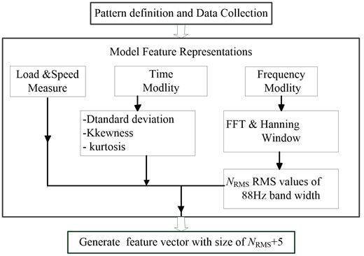
The time domain signal was multiplied by a Hanning window to obtain the FFT spectrum. The spectrum was divided in multiple bands, and the root mean square value (RMS) was calculated for each. The RMS value of each band is used as feature representation in the spectrum domain. With the objective of reducing the amount of input data the spectrum was split in multiple bands, because with this number of bands the root mean square (RMS) values keep track of the energy in the spectrum peaks [25]. RMS value is evaluated with Ep. (10), where $N$ is the number of samples of each frequency band:

10

${FFT}_{rms}=\sum _{n=1}^{N}FFT\left(n\right).$

Vectors of the features of the preprocessed signal are formed as follows: $N_{RMS}$ RMS values, standard deviation, skewness, kurtosis, rotation frequency and applied load measurements, which are used as input parameters for neural networks. The outline of feature representation of vibratory signals is as Fig. 4. In this work, the frequency range is 0 to 22050 Hz and the size of the data vector in the frequency is 18000 samples. The spectrum is divided in $N_{RMS}$ frequency bands, $N_{RMS}=$251.

Fig. 4Feature representation

4. Implemented classifier based on multi-layer neural network

4.1. Typical MLNN-based classifier

To validate the performance of the proposed MLNN_DBN-based classifier for gearbox fault diagnosis, we firstly implement the classifier based on typical MLNN. A batch training strategy is used to train the neural network, where the weights of nets are shared by a batch of training samples with mini batches of size. In other word, after training the neural network with a batch of samples, its errors, weights and biases are updated.

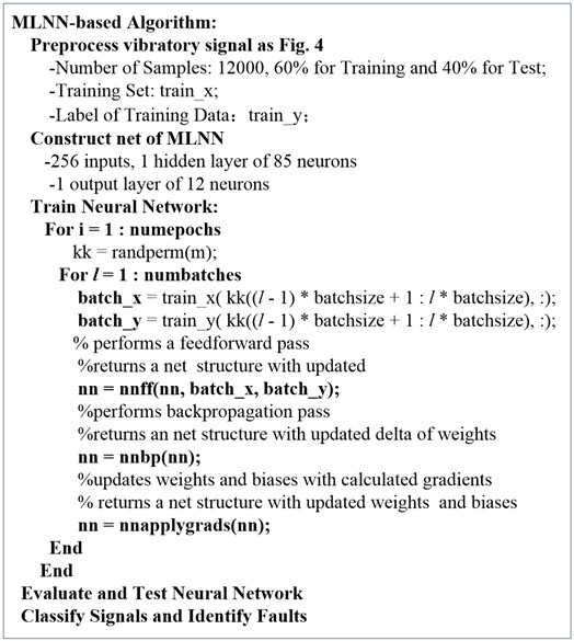
After performing a series of parameter tunings, a net of typical MLNN with 3 layers is constructed as follows: 256 inputs, 12 outputs, 1 hidden layer of 80 neurons, 1 output layer of 12 neurons; all neurons use the tan-sigmoid as the transfer function. The learning rate and momentum of the network are set to 2, 0.5, respectively. Activation function of hidden layers is $\mathrm{t}\mathrm{a}\mathrm{n}\mathrm{h}$ function, and that of output unit is sigmoid function. The size of batch training is 100. The number of samples is 12000. The number of iteration of training is 85. The training of the network is accomplished by using back propagation (BP) algorithm. The pseudo-code of the MLNN-based classifier is as Fig. 5.

Fig. 5Pseudo-code of MLNN-based classifier

5. Experimental setup

In this subsection, we firstly explain the gearbox fault diagnosis experimental platform. Fig. 7 indicates the internal configuration of the gearbox and positions for accelerometers. There are 3 shafts and 4 gears composing a two-stage transmission of the gearbox. An input gear ($Z_1=$ 27, modulus = 2, $\mathrm{\Phi }$ of pressure = 20) was installed on the input shaft. Two intermediate gears ($Z_2=Z_3=$ 53) were installed on an intermediate shaft for the transmission for the transmission between the input gear and the output gear ($Z_4=$ 80, installed on the output shaft). The faulty components used in the experiments included gears $Z_1$, $Z_2$, $Z_3$, $Z_4$, bearing $B_1$, $B_2$, $B_3$, $B_4$ as labeled in Fig. 7(a). Test’s conditions are described in the Table 1. The vibration signal is obtained from the measurements of a vertically allocated accelerometer in the gearbox case.

Fig. 6Pseudo-code of MLNNDBN-based classifier

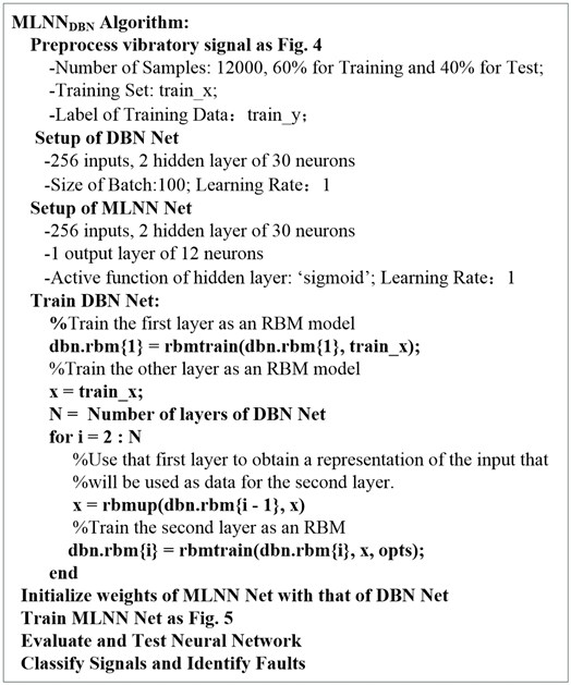
Fig. 7a) The internal configuration of the gearbox; b) positions for accelerometers

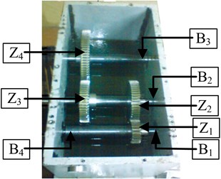
a)

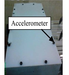
b)

Table 2 and 3 present the description of each fault condition of each component of the gearbox used in the experiment. We call them as basic condition pattern. In our experiment, a test case includes several basic condition patterns, which is a combination of multiple component faults. For example, the test case A shown in Table 4, includes following information of faults:

Gear $Z_1$: Gear with pitting on teeth;

Gear $Z_2$: Gear with face wear 0.5 [mm];

Bear $B_3$: Bearing with 4 pitting on outer ring;

Bear $B_2$: Bearing with 2 pitting on outer ring；

Gear $Z_4$ and $Z_3$, Bear $B_1$ and $B_4$: Normal.

To evaluate the performance of the proposed method for gearbox fault diagnosis, first, we constructed 12 condition patterns as listed in Table 4. Each pattern with 4 different load conditions and 5 different input speeds were applied during the experiments. For each pattern, load and speed condition, we repeated the tests for 5 times. In each time of the test, the vibratory signals were collected with 24 durations each of which covered 0.4096 sec.

In addition, to further validate the performance of the proposed approaches, a fault condition pattern library was constructed, which has 58 kinds of condition pattern based on the basis patterns described in Table 2 and Table 3. Each condition pattern has more than one basic gearbox fault. 20 test cases are used to test the robustness of the all MLNN-based methods; each test case has 12 kinds of condition pattern that are randomly selected from the pattern library.

6. Results and discussion

The training is done in first instance with the 12 patterns indicated in Table 4, using data with 12000 sample signals, where sixty percent of the samples set are used for the training of all MLNN-based approaches, and forty percent are used for testing. Table 5 shows their classification accuracy of the test case, including SVM classifier. We can see six MLNN-based approaches are effective for this test case, and are far better than SVM. The proposed MLNN_DBN has 98.1 % classification accuracy and is superior to other MLNN-based approaches.

One test case cannot reflect the reliability and robustness of an algorithm. So to further validate the performance of the proposed approach, a fault condition pattern library was constructed. 20 test cases are used to test the robustness of the all MLNN-based methods, where each test case has 12 kinds of condition pattern that are randomly selected from the defined pattern library.

The experiment results of 20 test cases using above described seven learning techniques respectively are shown in Table 6. Among 20 test cases, the MLNN (typical multi-layer neural networks) has 6 test cases with bad classification accuracy, although it is effective for other 14 test cases whose classification accuracies are larger than 90 %. The classification accuracy of MLNN are even smaller than SVM for 4 test cases (#1, #4, #7 and #13). It is obviously that typical MLNN gets easily stuck in “apparent local minima or plateaus” in some cases and has not good robustness for gearbox faults diagnosis.

Four fine-tuning schemes presented in subsection 2.2 (MLNN_Scheme1, MLNN_Scheme2, MLNN_Scheme3 and MLNN_Scheme4) improve obviously the performance of the typical MLNN. Compared with the typical MLNN, MLNN_Scheme1 has 13 test cases, MLNN_Scheme2 has 14 test cases, and MLNN_Scheme3 has 15 test cases to be superior to it. MLNN_Scheme4 only improves that of the typical MLNN in two test cases (#4 and #12). However, the classification rates of each fine-tuning scheme are smaller than 80 % for 5 test cases (#1, #4, #7, #13 and #20). They cannot still avoid falling into “apparent local minima or plateaus”.

Classification accuracies of MLNN_DBN for 20 test cases are presented in Table 6. The smallest one is 94.8 %, which is very excellent performance for gearbox fault diagnosis. Especially for the #1, #4, #7, #13 and #20 test case, the suggested MLNN_DBN has true positive classification rate larger than 96 %, in which other MLNN-based methods cannot all effectively classify them. The mean, standard deviation, least, and most value of classification rate for 20 test cases are also indicated in Table 6. Experiment results in Table 6 show MLNN_DBN achieves to avoid falling into “apparent local minima or plateaus”.

In addition, the MLNN_DBN method was compared with “shallow” learning algorithms SVM. As for the SVM, one of the most important representatives in the “shallow” learning community, good classification results can be found for the gearbox fault diagnosis, which is similar with some existing researches [26]. The algorithm SVM is applied using the LibSVM [27]. The parameters for SVM are chosen as $C=\text{1}$ and core (kernel) given by a radial basis $K\left(u,v\right)=\mathrm{e}\mathrm{x}\mathrm{p}(-\gamma {|u-v|}^2)$ function where $\gamma =\text{0.5}$. These parameters were found through a search, aiming at the best model for the SVM. Compared with other MLNN-based methods and SVM, we can see MLNN_DBN has most excellent performance and is highly reliable.

Fig. 8 shows the convergence process of error rate on the test case indicated in Table 4 for different MLNN-based classifiers. After about 20 epochs of training, the error rate of each method is less than 0.1. However, it is obviously to exist “overfitting” while undergo more than 20 epochs of training except for MLNN_DBN. Especially MLNN_scheme2 has serious “overfitting” after 60 epochs of training. From Fig. 8, we can see that MLNN_DBN is also robustness for gearbox fault diagnosis and overcome the problem of “overfitting”.

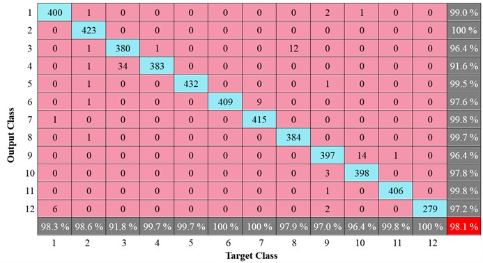
Confusion matrix is an effective and visualization tool of the performance of a classification algorithm. Each column of the confusion matrix represents the instances in a predicted class (output class), while each row represents the instances in an actual class (target class). Fig. 9 presents the confusion matrix using MLNN_DBN for 12 patterns indicated in Table 4. As shown in Fig. 9, it can be observed that the global percentage of true positive classification of the 12 condition patterns of faults is 98.1 % and the total error is 1.9 %. The smallest percentage of true positive classifications is obtained for type 3; this is because this kind of condition patterns with 6 basic faults. This is evident by observing the confusion matrix in which 34 times of type 4 are classified as type 3, noticing that mostly there is confusion between type 4 and type 3, in which they have 4 same basic faults. The percentage of true positive classification of Type 6, 7 and 12 are all 100 %. Confusion matrix in Fig. 9 shows the proposed MLNN_DBN has very high percentage of true positive classification for the test case.

Fig. 8The error rate on the test case indicated in Table 5 for different MLNN-based classifiers

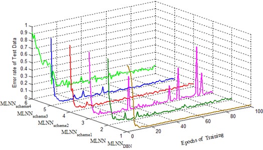
Fig. 9Confusion matrix using MLNNDBN

All above experiments indicate MLNN-based learning technologies are efficient and effective for gearbox faults diagnosis. Among them, MLNN_DBN has most effective performance and best robustness, which is highly reliable and applicable in fault diagnosis of industrial reciprocating machinery.

7. Conclusions

In this paper, multiple classifiers based on multi-layer neural network for the vibration measurements have been presented to diagnose the fault patterns of the gearbox. A MLNN-based learning architecture using deep belief network was proposed for gearbox fault diagnosis, which achieves to avoid falling into “apparent local minima or plateaus” and is highly reliable and applicable in fault diagnosis of gearbox. Other MLNN-based learning technologies are efficient and effective for gearbox faults diagnosis, however they may be fall into “apparent local minima or plateaus” in some cases. This type of classifiers could make a contribution to maintenance routines for industrial systems, towards lowering costs and guarantying a continuous production system, and with the appropriate equipment, online diagnostics could be performed. With these methods, complex fault combination with different component fault can be classified. These ways the implemented classifier could be utilized with ease in other kinds of rotating machinery in general for the classification and diagnostics of mechanical faults from their initial stages and in an extended range of cases, using the vibration signals, allowing this way to have the most efficient control and planning of maintenance of rotating machines. For evaluating the proposed MLNN-based methods, the gearbox fault diagnosis experiments were also carried out using SVM technique. The results show that the proposed MLNN_DBN-based methods are superior to SVM technique.