Abstract
For machinery product experienced several operating conditions, this paper proposes a framework of fuzzy reliability analysis of machinery accelerated testing. Due to the non-stationary of the vibration signals, a Gaussian mixture model (GMM) method is introduced to obtain the degradation index through calculating the overlap between current feature set and the historical baseline set. The features in four domains are extracted. Considered that the uncertainties exit in feature extraction and health assessment, a fuzzy regression model is used to describe the degradation path at each operating condition and compute fuzzy quasi time to failures (q-TTFs). Meanwhile, the relationship between q-TTFs and environmental variables are identified by a linear model, through which the fuzzy reliability analysis can be conducted with the most appropriate lifetime distribution. An industrial application is used to verify the effectiveness of the proposed framework and the results have confirmed a good consistency with the true values.
1. Introduction
In many engineering applications, such as airplanes, wind turbines and automobiles, rotating machinery parts are widely used and play a key role in their functions. Two commonly used machinery products are bearing and gear, which must have the attribute of high reliability [1]. The health monitoring of their status will not only prevent the unscheduled system downtime but also save related personnel and property losses. Thus, the research of condition-based maintenance (CBM) [1, 2] and prognostics and health management (PHM) [3] have being studied during the past decades. The purpose of the health monitoring is to tell that how far is the current state to system/component failure, i.e. remaining useful life (RUL), and make corresponding maintenance policy. A host of methods have been provided to conduct RUL prediction which are model-based, data-driven and hybrid models [1, 2, 4, 5].
The process of implementing CBM or PHM to machinery products is mainly consist of three aspects: data acquisition, data processing and maintenance decision support [2]. In general, the acquired data is vibration signal that cannot be directly used for RUL prediction, which is significantly different from electronic products or others whose degradation indexes are explicit, e.g. the light output of LEDs [6] and relative resistance in lithium-ion cells [7]. Although some statistical models can be applied to the vibration signals, there are still not a universal method. Thus, feature extraction methods are introduced to find the possible indexes that not be limited to time domain and can reflect the health status of the machinery products.
Feature extraction methods are also called signal processing techniques [2] that is to acquire health indexes from the raw vibration signals. The most common methods are time-domain, frequency-domain, time-frequency and information-domain analysis [8-10]. For example, Huang, et al. [11] obtained six vibration features from the ball bearing signals, which then are used to train the back propagation neural network and produce a performance degradation indicator for residual life prediction. Ocak, et al. [12] selected the node energies of decomposition tree as the features for bearing failure prognostics. In some applications, the features from the vibration signal cannot be selected as degradation indexes due to the dynamic and non-stationary properties of the vibration signal, which may be influenced by the uncertainties of the ambient environment or the complexity of machinery failure mechanism.
To solve above problem, a new aspect is proposed which considers that the machinery products are undergoing a gradual deterioration process. Thus, there must have some kind of difference between current status and historical health status using the extracted features. Liu, et al. [13] proposed a similarity-based method to quantitative the overlap between the distribution of the most recent status and the baseline health status and obtained an index named confidence value (CV) for health assessment. Following this idea, Liao, et al. [10] proposed a machine degradation assessment based on fixed cycle features test using Gaussian Mixture Model (GMM) and also used CV index to reflect the degradation status.
The literature of machinery health assessment mainly concentrates on specific eminent environment. While for product experienced different operating conditions [8, 14, 15], limited papers make research on identifying the influence of environment variables to the failure of the system or product and enhance their reliability level. Meanwhile, the uncertainties in feature extraction and health assessment should be considered since they may affect user’s belief on the assessment results. The uncertainties may originate from geometry [16], measurements [17] or degradation process modeling [18], etc.
Hence, based on abovementioned work, a framework of fuzzy reliability analysis of machinery accelerated testing is proposed in this paper. The paper is organized as follows: the proposed framework is given in Section 2. In Section 3, the features in four domains are obtained from raw vibration signals and the degradation indexes at each operating condition are acquired through GMM methods. In order to capture the inherent uncertainties in the degradation indexes, a fuzzy regression method is used to model the degradation path through which the fuzzy quasi time to failures (q-TTFs) are obtained in Section 4. Meanwhile, a linear model is provided to identify the relationship between q-TTFs and the operating conditions. In Section 5, the fuzzy reliability analysis is given with the selection of lifetime distribution. Section 6 illustrates an application of bearing accelerated degradation data from IEEE PHM 2012 data challenge to validate the effectiveness of the proposed framework in rotating machinery products. Discussions and conclusions are presented in Section 7 and 8.
2. The proposed framework of fuzzy analysis for machinery accelerated testing
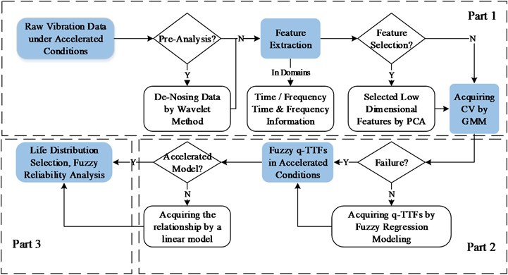
The proposed framework of fuzzy analysis of machinery accelerated testing is given in Fig. 1. The framework consists of three parts: degradation index acquisition, degradation modeling and fuzzy reliability analysis.
The first part is to obtain a degradation index from the raw vibration signals to reflect the health status of products. We at first de-noised the signals, if needed, by wavelet method to eliminate the extra influence of environmental noise. Then, the features in four domains, i.e. time, frequency, time-frequency and information domains, are extracted to obtain the overall information of products. Since the feature set is high dimensional, principal component analysis (PCA) method is introduced to reduce the dimension of the feature set based on the cumulated percentage of the principal components. After that, the GMM method is used to compute the degradation index by evaluating the overlap rate (CV) between the baseline features with the real-time ones. If the CV is near 1, the real-time health status is approximately normal, otherwise deterioration.
The second part is to model the degradation path of CV results and obtain the q-TTFs at each accelerated operating conditions. Due to the inherent uncertainties in feature extraction and health assessment, a fuzzy regression method is used to model the CV results with fuzziness and extrapolate the q-TTFs with the failure threshold. Before the fuzzy q-TTFs is used for reliability analysis, the acceleration model should be given to transfer the q-TTFs in accelerated operating conditions to normal ones. Thus, a linear model is used to find the relationship between the q-TTFs and the environmental variables. In addition, the contribution of each environmental variable or their combination to the failure of products can be expressed by the coefficients of the linear model.
The last part is to conduct fuzzy reliability analysis based on the fuzzy q-TTFs in normal operating condition, which can provide reliable information for maintenance decision-making through reliability, MTTF or other indexes. The following sections will address the analysis of accelerated testing with vibration data in detail.
Fig. 1The framework of fuzzy analysis of machinery accelerated testing
3. The degradation index
To implement the reliability prediction for machinery products which experience a gradual deterioration process that cannot be directly acquired from raw vibration data, feature extraction methods are used to find the degradation features. In general, one feature may be not enough to reflect the degradation status. For instance, the kurtosis factors from the vertical accelerometer signal is suitable for describing a gradual degradation for some bearings, but not for others [15]. Thus, the integration of multiple features is needed which can comprehensively reflect the degradation state of products. In this part, the degradation index CV is obtained by GMM method using features from four domains, which quantifies the overlap rate between current feature set (degradation status) and baseline set (normal status).
3.1. Feature extraction and principal component analysis
Feature extraction is to understand the performance of machinery product from the vibration signal at different aspect, which mainly includes time-domain, frequency-domain, time-frequency domain and information entropy as follows [2, 3].
3.1.1. Time-domain
The time-domain features present the transient variation of the vibration signal, which can directly reflect the health status of the products. In general, the features can be obtained from the statistical analysis, e.g. mean, variance, root mean square, peak, peak index, skewness, kurtosis, waveform, pulse and margin index, etc.
3.1.2. Frequency-domain
The frequency-domain features are transformed from the original time-domain signal using spectrum analysis, e.g. fast Fourier transform (FFT), to have a comprehensive understanding of the signal over the whole spectrum, e.g. the center frequency, mean square frequency and frequency variance.
3.1.3. Time-frequency domain
The time-frequency analysis method utilizes the strengths for both time-domain and frequency-domain analysis, and reflects the signal energy into two directions for the purpose of capturing fault pattern and conducting failure prognostics. In general, wavelet packet decomposition (WPD) and Hilbert-Huang transform (HHT) are widely used for time-frequency analysis. The energy of the first eight nodes from WPD method, which is decomposed into 4 layers with Daubechies wavelet as the mother wavelet, and HHT energy are selected as the features in this domain.
3.1.4. Information entropy
Information entropy is a measure of the uncertainty of the signal. A higher value indicates a higher uncertainty of the signal. Following this idea, the marginal spectrum entropy, HHT marginal spectrum entropy and HHT energy spectrum entropy are computed for feature analysis.
Assumed that signals are recorded during the experiment. The feature set is , where . To reduce the effect of different feature unit, is normalized into [0, 1] for each feature by, , and are the th row of feature set and its mean value.
The high dimensional feature set will led to the curse of dimensionality and cause heavy computational effort on the calculations. To facilitate the process of health assessment, PCA method [19] is introduced, which is a linear dimension reduction method through mapping the original set to a orthogonal space while minimizing the total squatted reconstruction error.
The × covariance matrix and its eigenvalue analysis are:
where, is the eigenvector, and is a diagonal matrix where the eigenvalues are in descending order. The cumulated percentage from eigenvalue 1 to is defined as. In engineering applications, it is acceptable to reduce the feature dimension with a value around [0.8, 0.9], while 0.8 is used in this paper. Then, the reduced × dimensional feature set can be given by Eq. (2):
3.2. Acquiring degradation index through GMM method
Based on the new dimensional feature set, the next step is to acquire the degradation index. For bearings, a gradual deterioration may happen due to ball wearing or inner impurity particles, which means that the extracted features should present the changing process. For instance, during the first monitor intervals, the tested product is in health status. With the time goes on, the most recent intervals should be in a partially degradation status. Following this idea, a GMM modeling method is introduced to obtain the degradation index through the measure of overlap rate [10, 20, 21].
Supposed that present one status with the columns of feature set . The probability density function (PDF) of, , follows a mixture distribution with Gaussian components that is:
where, is the weight of the th mixture and is:
Through the expectation maximization (EM) algorithm, the values of unknown parameters, i.e., , , will be obtained when the likelihood function value is converged or the number of iteration reaches the maximum [10, 22].
3.3. Basic EM algorithm for the estimation of GMM model parameters
1) , initialize the unknown parameters for all Gaussian components, , , .
2) do .
step: compute the posterior probability of sample of in the th component:
step: update , and :
3) end if or .
Therefore, the GMM model for each -interval (i.e. one health state) can be computed through abovementioned algorithm. The confidence value (CV) between the baseline model (i.e. normal state) and the most recent th model can then be calculated by the overlap between two GMM models [10, 23]:
If the th state is still in normal, the CV value will be near 1. Otherwise, it will be near 0 if the th state is barely normal which indicates the corresponding maintenance should be given to avoid the system failure. Hence, the CV results can be used as the degradation index for machinery product health assessment.
4. Degradation modeling and acceleration model
Given the degradation index from the vibration data under different operating conditions, the assessment of reliability and lifetime for machinery products can be conducted after extrapolating q-TTFs based on the degradation index. In this paper, we consider the uncertainties from information loss when acquiring features from raw vibration data, and CV calculation by Mahalanobis distance (M-D). The inherent uncertainties are not negligible since that they have influence on the credibility of the user’s belief on the reliability and lifetime assessment results. Thus, the fuzzy regression method is used to model the degradation paths for CV results with fuzzy theory. Similar applications are referred to [17, 18].
In this section, the basic fuzzy arithmetic is at first introduced for fuzzy calculations. Then, the modeling process using fuzzy regression model is illustrated in order to obtain the fuzzy q-TTFs at different operating conditions. After that, the acceleration model is identified to establish the relationship between failure times and operating conditions since the reliability prediction is conducted at normal operating condition.
4.1. Basic fuzzy arithmetic
Zadeh [24] introduced fuzzy set theory to solve the problem of uncertainty due to imprecise or vague through applying a membership function to data rather than crisp one. Membership functions, e.g. triangular, rectangular or trapezoidal, are widely used. Without loss of generality, triangular membership function is selected to simply the calculations. Let be a fuzzy number with triangular membership function, see Fig. 2. Herein, , and donate the center, left boundary and right boundary, respectively. The presents the membership value of in, i.e.:
Fig. 2Fuzzy number and its alpha-cuts
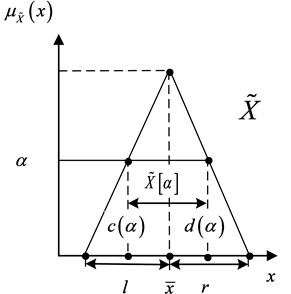
The realization of fuzzy numbers are always conducted with alpha-cuts, which decomposes the membership function at the vertical axis with membership value (see Fig. 2), i.e. . The alpha-cuts of is defined as:
where, and are increasing and decreasing function of with [25]. When , [ is called the support of fuzzy number .
Assuming two triangular numbers and with their alpha-cuts, namely and , the operator can be calculated with basic interval arithmetic and alpha-cuts. The results of addition, subtraction, multiplication and division between two fuzzy numbers are , , and , respectively. Provided that zero does not belong to for all in division [18, 25]. Assuming a function is , is a fuzzy function and the membership function of can be calculated through Zadeh’s extension principle, i.e.
If is continuous, then the alpha-cuts for , namely , are [26]:
4.2. Fuzzy regression method and q-TTFs
For the analysis of imprecise degradation data, fuzzy regression method is a powerful tool to model the degradation path containing the epistemic uncertainty by means of fuzzy theory. There are two options when using this method to model the degradation path. The first one utilizes a membership function to each degradation data. Then, the regression method with fuzzy parameters is used to model the degradation path [17, 27]. The second one directly uses the regression method to model the degradation path and select the (1-) 100 % confidence intervals of the parameters as their fuzzy estimators [18]. Taking the CV results in Section 3.2 as an example, the data are imprecise because of the inherent uncertainties. Since no prior information is given to establish the membership function for CV results, the second method is selected in this paper.
In general, the degradation paths can be classified into three types: linear, convex and concave. Thus, the linear, exponential and power law relationships are widely used for degradation modeling. And, the basic regression model is defined as:
where, is the expected degradation path, is the constant parameters, is the error term which follows normal distribution. Herein, one may use the statistical fitting indexes to select the most appropriate degradation model among the three candidate models in Eq. (12), e.g. and . Meanwhile, the unknown parameters of the selected degradation model can be estimated through least square method.
Then, the (1-) 100 % confidence interval for vector parameters are regarded as the fuzzy estimators for parameters , which is [18]:
where, is the number of CV results, is the number of unknown parameters which is equal to 2. For the sake of simplicity, the symmetric triangular membership function is selected for fuzzy parameters, i.e. in Eq. (8), and their alpha-cuts are defined as for all .
Thus, the fuzzy regression model is:
When the failure threshold is available, the corresponding fuzzy failure time at each operating condition will be computed at each alpha-cut using interval arithmetic.
4.3. Acceleration model
The machinery products are experienced with hasher than normal conditions. In order to evaluate the lifetime and reliability results at normal operating condition, the relationship between q-TTFs and accelerated conditions should be obtained through acceleration model.
Generally, acceleration models are given through physical mechanism analysis or empirical experiences. Examples include Arrhenius model, Eyring model or inverse power model [28]. When no prior knowledge is acquired for machinery products, like the bearing under different load and speed conditions, the following log-linear relationship is recommended. Similar application can be found in [29]:
where, is the coefficient, 1, 2,…,5, and donate speed and load for bearing operating conditions, is the failure time. The optimal parameters for Eq. (15) can be obtained through least square method by “fitlm” function in Matlab. Similarly, the fuzzy acceleration model can be given to describe the relationship between the environmental variables, i.e. load, speed, and the fuzzy q-TTF under each alpha-cut for all .
Then, under each alpha-cut, the averaged fuzzy q-TTFs at both normal operating condition and the th stress level, i.e. and , can be computed by substituting the corresponding speed and load into the optimal function. Therefore, the fuzzy acceleration factor (AF) is defined as:
With the results from Eq. (16), fuzzy q-TTFs can be extrapolated to normal operating condition .
Besides the lifetime and reliability evaluation, another advantage of accelerated testing is that it can provide information about the stresses or their combinations which are sensitive to the failure of machinery products. Such information can provide reliable basis for reliability growth and design improvement for products. The following algorithm is proposed for such purpose through the analysis of fuzzy coefficients .
4.4. Analysis of sensitive stresses
Set , which denotes the number of intervals for membership value in [0, 1].
1) , compute the fuzzy coefficient at each alpha-cut .
Substitute all fuzzy failure time and its corresponding th condition and :
;
;
;
;
Compute fuzzy acceleration factor through Eq. (16).
2) End if .
3) Construct membership function for all fuzzy coefficient and analyze the relationship between them, compute the main stress.
5. Lifetime distribution selection and fuzzy reliability analysis
In this section, a procedure of lifetime distribution selection is proposed for fuzzy q-TTFs under normal operating conditions. Then, the fuzzy reliability analysis is conducted with the most appropriate distribution to compute indexes that of interest, e.g. reliability, MTTF, etc.
5.1. Lifetime distribution for q-TTFs
In order to select the lifetime distribution under fuzzy q-TTFs, Anderson-Darling test [30] is used to test the goodness of fit of the candidate distribution to the obtained q-TTFs at each alpha-cut. The following procedure is proposed to rank the candidate distributions which are normal, exponential, extreme value, Log-normal and Weibull distributions.
1) Set, which denotes the total score of the th distribution at all alpha-cuts in [0, 1], and the significance level (default is 5 %).
2) , compute the fuzzy coefficient at each alpha-cut .
Calculate the score whether A-D test reject the null hypothesis that failure times are from the th distribution.
;
If yes,, ; else , .
3) End if .
4) Rank the in an ascending order and select the lowest (or the first) one as the most appropriate lifetime distribution.
For some specific applications, like bearings, studies have shown that the failure times follow Weibull distribution [31] which can be directly used for fuzzy reliability analysis:
where, is scale parameter, and is shape parameter. In classical reliability engineering, 1 means that the product experiences a wear-out phase from the perspective of the bathtub curve. For fuzzy q-TTFs, the fuzzy parameters, i.e. and , are estimated through lifetime distribution fitting for at each alpha-cut.
5.2. Fuzzy reliability analysis
The selected lifetime distribution can then be used for reliability prediction. The fuzzy reliability at time interval [, ] is defined as (Weibull distribution as an example):
Other reliability indexes, e.g. Mean Time to Failure (MTTF) or hazard function, can compute through substituting fuzzy parameters into classical analytical results at each alpha-cut:
Furthermore, if other lifetime distribution is satisfied, e.g. Log-normal distribution, Eqs. (18) and (19) can be rewritten accordingly.
6. Case study
In this section, an industrial application is used to illustrate the feasibility of the proposed method.
6.1. Experiment platform
The analyzed data is from IEEE PHM 2012 data challenge and the bearing experiment platform PRONOSTA is shown in Fig. 3, which is consist of three parts: the rotating, degradation generation and measurement parts [15]. The sampling frequencies are 25.6 kHz for the embedded acceleration measures and 10 Hz for temperature ones. The platform can perform bearing accelerated degradation testing, while monitoring vibration and temperature signals for fault diagnosis and remaining useful life (RUL) prediction.
Fig. 3The bearing experiment platform [17]
![The bearing experiment platform [17]](https://static-01.extrica.com/articles/15970/15970-img3.jpg)
The tested 17 bearings are experienced three operating conditions with different rotating speed and load, i.e. 1800 rpm and 4000 N (Condition 1), 1650 rpm and 4200 N (Condition 2) and 1500 rpm and 5000 N (Condition 3) and the bearing failure happens when the accelerometer exceeds 20 g. Table 1 gives the details about the tested bearings which are divided into two sets for training and testing (algorithms or models). Due to the inner non-linear property for bearing features, it is quite difficult to accurately estimate the RULs [15, 32]. Hence, the proposed framework is used to conduct bearing reliability analysis with accelerated data. Since the bearing reliability is an index for the population but not individual, the bearings whose lifetimes are significant lower or higher than others are omitted, i.e. 1_2, 1_4, 2_1, 2_7. In addition, the vibration signals from vertical axis is selected since it has been verified to be better reflect the health state [33].
Table 1Datasets of the bearing accelerated testing
Datasets | Operating conditions | ||
Condition 1 | Condition 2 | Condition 3 | |
Learning set | No. 1_1 | No. 2_1 | No. 3_1 |
No. 1_2 | No. 2_2 | No. 3_2 | |
Testing set | No. 1_3 | No. 2_3 | No. 3_3 |
to | to | ||
No. 1_7 | No. 2_7 | ||
6.2. Degradation modeling and fuzzy q-TTFs
According to the procedure in Section 2, the original signal is at first de-noised by the wavelet method at level 4 using the principle of Stein’s unbiased risk with soft-thresholding [34]. Then, the 25 features in four domains are extracted and then reduced through PCA method where 0.8. After that, the degradation index CV can be obtained using GMM method in Section 3.2. Herein, the choice for the number of features as one state needs more attention, especially for the baseline normal state. We used different combination of values in three operating conditions and compared their CV results with the announced bearing failure in the learning set, where the acceleration level exceeds 20 g. Thus, 1100, 300 and 250 are selected as one health state for three conditions. In addition, the new failure threshold for the degradation index is set to 0.2, i.e. 0.2. The GMM results are shown in Fig. 4.
Fig. 4The degradation processes for bearings under three accelerated levels with their fitted paths
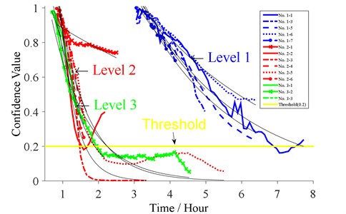
Then, three degradation models given in Eq. (12) are used to model the path of CV results at each operating condition. The fitting results are listed in Table 2. The linear model gives bad fitting results for bearing 2_3, 2_5, 2_6 although it performs well for other bearings. Meanwhile, Fig. 4 shows that the degradation processes are non-linear. For the other two models, the exponential model is selected with larger and values than power model for most of the bearings, which will be used for the following q-TTF extrapolation.
Table 2Model comparison for degradation modeling
Bearing no. | linear | exponential | power | |||
(%) | (%) | (%) | (%) | (%) | (%) | |
1_1 | 96.2 | 96.1 | 95.4 | 95.3 | 90.6 | 90.4 |
1_3 | 92.9 | 92.6 | 87.2 | 86.6 | 83.0 | 82.2 |
1_5 | 98.3 | 98.3 | 95.2 | 95.1 | 90.9 | 90.7 |
1_6 | 98.2 | 98.2 | 98.5 | 98.4 | 96.2 | 96.1 |
1_7 | 94.8 | 94.4 | 93.5 | 93.0 | 92.1 | 91.4 |
2_2 | 96.1 | 95.6 | 93.8 | 93.0 | 89.9 | 88.7 |
2_3 | 61.3 | 60.0 | 91.8 | 91.5 | 86.5 | 86.0 |
2_4 | 96.8 | 96.4 | 90.9 | 89.9 | 85.3 | 83.7 |
2_5 | 48.2 | 47.3 | 86.7 | 86.5 | 90.8 | 90.6 |
2_6 | 98.6 | 98.4 | 94.1 | 93.4 | 89.7 | 88.4 |
3_1 | 96.9 | 96.4 | 92.6 | 91.5 | 87.2 | 85.4 |
3_2 | 62.0 | 61.1 | 91.8 | 91.6 | 96.9 | 96.9 |
3_3 | 97.2 | 95.8 | 96.8 | 95.2 | 95.6 | 93.3 |
The statistical results for the selected exponential degradation model are given in Table 3, where Anderson-Darling test is used to check the normal assumption of the error term. Hence, the degradation paths for bearings No. 1_3, 2_3, 2_5 and 3_2 are not compromised with the normal assumption although the and suggest good fitting. As seen from Fig. 4, the bearing 1_3 experienced a sudden decrease and it will fail soon which is not accordance with others in operating condition 1. Thus, the bearing 1_3 is omitted for the following analysis. In terms of bearings No. 2_3, 2_5 and 3_2, the CV values are already lower than the failure threshold 0.2 around 2 (h). Considered that the tails of the degradation paths present a state that is much deviate from the normal state. The CV results are ignored from time 1.5, 2 and 2.111(h) from the three bearings. As to bearing 2_2, it seems to perform better after 1.5833 (h) which, however, has already exceeded the threshold. Thus, the CV values after 1.5833 (h) are ignored for bearing 2_2. The new results for this four bearings are given in Table 3 by adding a bracket, e.g. [2_3].
The fuzzy parameters of the exponential degradation model are constructed as illustrated in Section 4.2. The 95 % confidence values are shown at the right of Table 3. For simplicity, the symmetrical triangle membership function is selected to present the belief of certain parameter through the membership values. Thus, the fuzzy q-TTFs can be computed by substituting fuzzy parameters, i.e. and , and the failure threshold 0.2 into Eq. (14) at each alpha-cut, which are interval values as . The results are given at the left side of Table 4.
Table 3Fuzzy results for exponential degradation model parameters
Bearing no. | AD (error) | Fuzzy estimation | ||||||||
SE | SE | stat | ||||||||
1_1 | 3.389 | 0.189 | –0.367 | 0.013 | 0.070 | 0.68 | 3.031 | 3.788 | –0.393 | –0.342 |
1_3 | 3.461 | 0.433 | –0.377 | 0.033 | 0.011 | 0.98 | 2.670 | 4.486 | –0.452 | –0.315 |
1_5 | 3.646 | 0.244 | –0.402 | 0.016 | 0.051 | 0.74 | 3.185 | 4.175 | –0.436 | –0.370 |
1_6 | 2.376 | 0.057 | –0.264 | 0.006 | 0.189 | 0.51 | 2.264 | 2.494 | –0.276 | –0.253 |
1_7 | 2.648 | 0.225 | –0.312 | 0.024 | 0.423 | 0.35 | 2.200 | 3.187 | –0.369 | –0.264 |
2_2 | 3.314 | 0.922 | –1.483 | 0.243 | 0.598 | 0.29 | 1.832 | 5.997 | –2.102 | –1.046 |
[2_2] | 6.421 | 1.521 | –2.143 | 0.232 | 0.494 | 0.32 | 3.719 | 11.09 | –2.752 | –1.669 |
2_3 | 8.164 | 1.833 | –2.278 | 0.217 | 0.003 | 1.20 | 5.157 | 12.92 | –2.767 | –1.876 |
[2_3] | 3.625 | 1.109 | –1.668 | 0.337 | 0.457 | 0.33 | 1.759 | 7.471 | –2.691 | –1.035 |
2_4 | 3.046 | 0.483 | –1.217 | 0.142 | 0.685 | 0.26 | 2.128 | 4.360 | –1.584 | –0.935 |
2_5 | 2.796 | 0.311 | –1.176 | 0.086 | 8e-04 | 1.46 | 2.237 | 3.495 | –1.363 | –1.015 |
[2_5] | 2.753 | 0.307 | –1.319 | 0.109 | 0.062 | 0.68 | 2.163 | 3.505 | –1.576 | –1.104 |
2_6 | 4.309 | 0.742 | –1.629 | 0.162 | 0.874 | 0.20 | 2.897 | 6.410 | –2.049 | –1.294 |
3_1 | 2.200 | 0.251 | –1.054 | 0.120 | 0.256 | 0.43 | 1.679 | 2.882 | –1.378 | –0.806 |
3_2 | 1.862 | 0.134 | –0.995 | 0.057 | 0.010 | 1.01 | 1.611 | 2.152 | –1.117 | –0.886 |
[3_2] | 2.436 | 0.073 | –1.258 | 0.028 | 0.558 | 0.31 | 2.286 | 2.595 | –1.319 | –1.200 |
3_3 | 1.555 | 0.108 | –0.659 | 0.086 | 0.152 | 0.43 | 1.153 | 2.098 | –1.152 | –0.377 |
Table 4Fuzzy q-TTFs under accelerated and normal conditions
Bearing no. | Fuzzy q-TTFs | Operating conditions | Fuzzy q-TTFs in normal condition (3000 rpm, 1200 N) | |||
(h) | (h) | Speed (rpm) | Load (N) | (h) | (h) | |
1_1 | 6.9177 | 8.6064 | 1800 | 4000 | 10.6271 | 22.0470 |
1_5 | 6.3450 | 8.2060 | 9.7474 | 21.0214 | ||
1_6 | 8.8065 | 9.9668 | 13.5288 | 25.5319 | ||
1_7 | 6.5015 | 10.496 | 9.9878 | 26.8877 | ||
2_2 | 1.0621 | 2.4053 | 1650 | 4200 | 5.2697 | 35.8368 |
2_3 | 0.8079 | 3.4998 | 4.0082 | 52.1441 | ||
2_4 | 1.4923 | 3.2946 | 7.4040 | 49.0869 | ||
2_5 | 1.5105 | 2.5948 | 7.4940 | 38.6610 | ||
2_6 | 1.3044 | 2.6794 | 6.4715 | 39.9207 | ||
3_1 | 1.5441 | 3.3117 | 1500 | 5000 | 6.0995 | 36.8122 |
3_2 | 1.8473 | 2.1364 | 7.2975 | 23.7476 | ||
3_3 | 1.5210 | 6.2316 | 6.0083 | 69.2690 | ||
6.3. Acceleration model and analysis of sensitive stresses
After obtaining the fuzzy q-TTFs under three operating conditions, Eqs. (15) and (16) in Section 4.3 can then compute the fuzzy acceleration factors (see Fig. 5) with their fuzzy coefficients, and convert the failure times into normal operating conditions. Assumed that the normal condition is 3000 (rpm) in Speed and 1200 (N) in load, the results are given at the right side of Table 4.
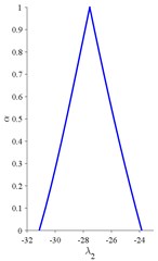
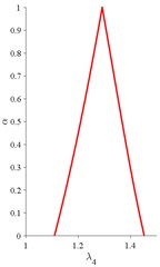
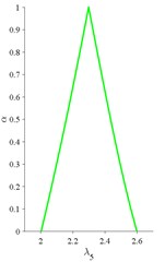
From Fig. 5, it can conclude that the support of fuzzy acceleration factors under three acceleration operating conditions are [1.53, 2.56], [4.96, 14.90] and [3.95, 11.12], while the peak values are 2.44, 10.57 and 8.58, respectively. Intuitively, both condition 2 & 3 are harsher than condition 1 with larger values of acceleration factor under each alpha-cut for all . And condition 2 is severer than condition 3 when the belief of the results 0.8, otherwise their difference are undistinguishable. Furthermore, the fuzzy coefficients of the acceleration model can be used to analyze the sensitivity of speed and load to the lifetimes of bearings through the procedure in Section 4.3. The results show that, and are zero for all which means that no contribution to the failure of bearings has been obtained for the single stress of speed and the interactive stress of speed and load. Thus, the sensitive stresses are load, self-correlation of speed and load, which are related to coefficient, and, see Fig. 6. The results can help understand the hazard rating for each stress or their combination to the failure of bearings, and improve the design or operating conditions to increase the lifespan of bearings.
Fig. 5Fuzzy acceleration factors for three accelerated operating conditions
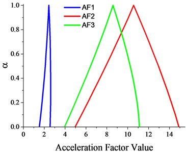
Fig. 6Fuzzy coefficients in acceleration models
a)
b)
c)
6.4. Lifetime distribution selection and fuzzy reliability analysis for bearings
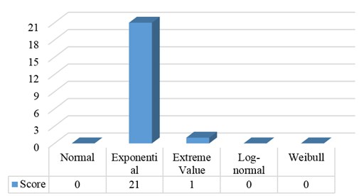
Once the fuzzy q-TTFs are given, the selection of lifetime distribution is essential for reliability analysis. In this case, the procedure of distribution selection proposed in Section 5.1 is used to compute the score of each candidate distribution for fuzzy q-TTFs at both sides. The membership value is equally divided into 10 intervals, which means that 10 and the maximum score will be. Fig. 7 presents the results and indicates that normal, Log-normal and Weibull distributions are appropriate for describing bearing lifetime data, while exponential distribution is not suitable at all and extreme value distribution seems well with only one score. Although it has been demonstrated that the failure times for bearing follows Weibull distribution [31], the normal and Log-normal distributions also perform well in this study. The reason may be from the small sample (12 bearing lifetime data), which leads to the similar shape that those three distributions can describe. Thus, special attention should be given for other applications if there have no such prior knowledge. For bearings, the Weibull distribution is used for computing fuzzy reliability and MTTF.
Fig. 7The score of each distribution for bearing failure times
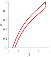
The fuzzy parameter for Weibull distribution is calculated at each alpha-cut, see Fig. 8. For all , is greater than 1 which means that the bearing experienced a wear-out phase. Interested that with different belief of the results, the fuzzy value varied from [2.80, 3.25] to the peaking 9.30. That is to say, with different belief, the recognition on the severity of bearing deterioration is significantly different. While in traditional analysis, only one crisp value can be obtained and such phenomenon cannot be identified.
Fig. 8Fuzzy parameters for the Weibull lifetime distribution
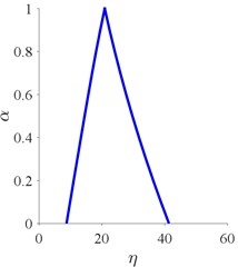
As described in the challenge details [15], the lifetimes for the majority of the bearings are from 1 to 7 (h). It may be interesting to analyze the reliability of this kind of bearing during the next hour in normal operating condition. Thus, the time interval [7, 8] (h) is substituted to Eq. (18) with fuzzy Weibull parameters. Fig. 9 shows the results, where the reliability results is in [0.8573, 0.9969] and have the peak value at 0.9999. The results demonstrate that the bearings have a higher possibility that is safety enough for operating under normal operating condition.
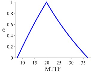
For users, the maintenance time is that of interest for making schedule to avoid the occurrence of failure and reduce their related costs. Hence, the fuzzy MTTF values is then computed using Eq. (19), see Fig. 10. The MTTF goes from 7.83 to 36.82 (h) and have the highest peak at 19.83 (h). In this case, it has the lowest possibility that maintenance schedule should be given before 7.83 (h), while the highest at 19.83 (h). Compared with traditional crisp value, the related risk can be directly expressed by fuzzy MTTF. For instance, if the traditional value is at the left side of fuzzy MTTF, the schedule will be conservative. Otherwise, it will be radical.
Fig. 9Fuzzy reliability for bearings at time interval [7, 8] (h)
![Fuzzy reliability for bearings at time interval [7, 8] (h)](https://static-01.extrica.com/articles/15970/15970-img12.jpg)
Fig. 10Fuzzy MTTF for bearings
7. Verification and discussion
For the proposed framework, it may be interesting to verify its effectiveness through actual failure time data from two aspects. On the one hand, the comparison between fuzzy q-TTFs obtained from the regression method and the actual ones (see Table 5) is to verify that the extracted degradation index, i.e. CV results, can be used for lifetime prediction. On the second hand, the comparison between reliability and MTTF results from the proposed method and that from the actual data will further verify that the proposed can well handle the risk of the reliability prediction results.
All the tested 17 bearings were ran to failure, which can be found in http://www.femto-st.fr/ieee-PHM2012-data-challenge. The actual failure times are summarized at the left of Table 5. Among that, 12 bearings are selected for reliability analysis and the fuzzy q-TTFs are given in Table 4. Through comparison, it can conclude that the failure times of 5 bearings are in the intervals of fuzzy results, i.e. 1_1, 1_5, 2_2, 2_4 and 2.6, while 4 bearings are slightly overestimated, i.e. 1_6, 1_7, 3_1 and 3_2, the 3 rest bearings are underestimated. Thus, the proposed method perform well on lifetime prediction for bearings using the degradation index obtained from GMM method.
Now, before conducting reliability analysis, it is necessary to identify the acceleration model. Herein, Eq. (15) is used and the result is:
Thus, the main sensitive stresses are load, self-correlation of speed and load, which are in good agreement with the results from the proposed method in Section 6.3. In addition, the acceleration factors for the three accelerated operating conditions are 4.71, 8.31 and 9.70. As seen from Fig. 5, the fuzzy results well capture Condition 2 & 3, while underestimate the Condition 1. Considered that the complexity of the interaction among the associated uncertainties, the results are acceptable. The extrapolated TTFs under normal operating condition are listed at the right side of Table 5. Anderson-Darling test shows that the Weibull distribution is a suitable lifetime distribution.
In the next step, we compare the reliability and MTTF results. The scale and shape values for Weibull distribution are 28.93 and 2.04. Substituting them into Eq. (18), the reliability for the bearings at [7, 8] (h) is 0.9837. It is obvious that the fuzzy result from the proposed method can well present the value, see Fig. 9. Moreover, the proposed method can tell that the reliability is more than 0.8573 even in the worst-case. Similarly for MTTF, the result is 25.63 (h) which is well presented by the proposed method in Fig. 10.
From above analysis, it concludes that the proposed framework can provide reliable reliability and MTTF results for bearings and consider the uncertainties with related risk in accelerated data. The proposed framework can be applied to the lifetime prediction and reliability evaluation for other machinery applications with accelerated data.
When implementing the proposed framework, special attention should be given to the elimination of noises from the raw vibration signals, which may be originated from the operating environment contaminated by noises, and have effect on the results of lifetime evaluation and reliability prediction. Therefore, the de-nosing methods should be chosen with carefully consideration for one specific machinery product, e.g. the wavelet method given in Fig. 1.
Table 5Actual TTFs for all bearings at accelerated and normal operating conditions
Bearing no. | TTFs (Accelerated condition) (h) | Operating conditions | TTFs (3000 rpm, 1200 N) (h) | |
Speed (rpm) | Load (N) | |||
1_1 | 7.7833 | 1800 | 4000 | 36.6260 |
1_2 | 2.4167 | 11.3721 | ||
1_3 | 6.5944 | 31.0315 | ||
1_4 | 3.2553 | 15.3184 | ||
1_5 | 6.8389 | 32.1817 | ||
1_6 | 6.7969 | 31.9844 | ||
1_7 | 6.2725 | 29.5165 | ||
2_1 | 2.5278 | 1650 | 4200 | 21.0158 |
2_2 | 2.2111 | 18.3831 | ||
2_3 | 5.4278 | 45.1263 | ||
2_4 | 2.0833 | 17.3207 | ||
2_5 | 6.4167 | 53.3479 | ||
2_6 | 1.9444 | 16.1660 | ||
2_7 | 0.6361 | 5.2886 | ||
3_1 | 1.4278 | 1500 | 5000 | 13.8529 |
3_2 | 4.5444 | 44.0921 | ||
3_3 | 1.2028 | 11.6699 | ||
8. Conclusions
This study has focused on the fuzzy reliability analysis of machinery accelerated testing data. A framework has been proposed which consists of three aspects: degradation index acquisition, degradation modeling and fuzzy reliability analysis. The proposed framework can compute reliable reliability and MTTF results for maintenance decision-making.
The GMM method can use a mixture of Gaussian distributions to capture one status of machinery product by extracting features from raw vibration signals. This method can derive a health status even though the signals are dynamic and non-stationary. A linear model is used to identify the relationship between environmental variables and TTFs. For the case study, it has confirmed that the main sensitive stresses of bearing failure are load, self-correlation of speed and load. During the comparison with real failure data, the proposed method can capture the real values well. Meanwhile, the fuzzy results of reliability and MTTF verified the advantages of the proposed method to understand the potential risk of the acceptance of the results.
References
-
Heng A., Zhang S., Tan A. C. C., Mathew J. Rotating machinery prognostics: state of the art, challenges and opportunities. Mechanical Systems and Signal Processing, Vol. 23, Issue 3, 2009, p. 724-739.
-
Jardine A. K. S., Lin D. M., Banjevic D. A review on machinery diagnostics and prognostics implementing condition-based maintenance. Mechanical Systems and Signal Processing, Vol. 20, Issue 7, 2006, p. 1483-1510.
-
Lee J., Wu F. J., Zhao W. Y., Ghaffari M., Liao L. X., Siegel D. Prognostics and health management design for rotary machinery systems – reviews, methodology and applications. Mechanical Systems and Signal Processing, Vol. 42, Issues 1-2, 2014, p. 314-334.
-
Sikorska J. Z., Hodkiewicz M., Ma L. Prognostic modelling options for remaining useful life estimation by industry. Mechanical Systems and Signal Processing, Vol. 25, Issue 5, 2011, p. 1803-1836.
-
Si X. S., Wang W. B., Hu C. H., Zhou D. H. Remaining useful life estimation – a review on the statistical data driven approaches. European Journal of Operational Research, Vol. 213, Issue 1, 2011, p. 1-14.
-
Wang F. K., Lu Y. C. Useful lifetime analysis for high-power white LEDs. Microelectronics Reliability, Vol. 54, Issues 6-7, 2014, p. 1307-1315.
-
Thomas E. V., Bloom I., Christophersen J. P., Battaglia V. S. Statistical methodology for predicting the life of lithium-ion cells via accelerated degradation testing. Journal of Power Sources, Vol. 184, Issue 1, 2008, p. 312-317.
-
Şeker S. A reliability model for induction motor ball bearing degradation. Electric Power Components and Systems, Vol. 31, Issue 7, 2003, p. 639-652.
-
Williams T., Ribadeneira X., Billington S., Kurfess T. Rolling element bearing diagnostics in run-to-failure lifetime testing. Mechanical Systems and Signal Processing, Vol. 15, Issue 5, 2001, p. 979-993.
-
Liao L., Lee J. A novel method for machine performance degradation assessment based on fixed cycle features test. Journal of Sound and Vibration, Vol. 326, Issues 3-5, 2009, p. 894-908.
-
Huang R., Xi L., Li X., Liu C. R., Qiu H., Lee J. Residual life predictions for ball bearings based on self-organizing map and back propagation neural network methods. Mechanical Systems and Signal Processing, Vol. 21, Issue 1, 2007, p. 193-207.
-
Ocak H., Loparo K. A., Discenzo F. M. Online tracking of bearing wear using wavelet packet decomposition and probabilistic modeling: a method for bearing prognostics. Journal of Sound and Vibration, Vol. 302, Issues 4-5, 2007, p. 951-961.
-
Liu J., Djurdjanovic D., Ni J., Casoetto N., Lee J. Similarity based method for manufacturing process performance prediction and diagnosis. Computers in Industry, Vol. 58, Issue 6, 2007, p. 558-566.
-
Seker S., Ayaz E. Feature extraction related to bearing damage in electric motors by wavelet analysis. Journal of the Franklin Institute, Vol. 340, Issue 2, 2003, p. 125-134.
-
Nectoux P., Gouriveau R., Medjaher K., Ramasso E., Morello B., Zerhouni N., Varnier C. PRONOSTIA: An experimental platform for bearings accelerated life test. IEEE International Conference on Prognostics and Health Management, Denver, USA, 2012.
-
Most T., Knabe T. Reliability analysis of the bearing failure problem considering uncertain stochastic parameters. Computers and Geotechnics, Vol. 37, Issue 3, 2010, p. 299-310.
-
Wang Z., Huang H.-Z., Du L. Reliability analysis on competitive failure processes under fuzzy degradation data. Applied Soft Computing, Vol. 11, Issue 3, 2011, p. 2964-2973.
-
Gonzalez-Gonzalez D. S., Alejo R. J. P., Cantu-Sifuentes M., Torres-Trevino L. M., Mendez G. M. A non-linear fuzzy regression for estimating reliability in a degradation process. Applied Soft Computing, Vol. 16, 2014, p. 137-147.
-
Jolliffe I. Principal Component Analysis. Wiley Online Library, 2005.
-
Reynolds D. Gaussian Mixture Models. Encyclopedia of Biometrics, 2009, p. 659-663.
-
Qiu L., Yuan S., Chang F.-K., Bao Q., Mei H. On-line updating Gaussian mixture model for aircraft wing spar damage evaluation under time-varying boundary condition. Smart Materials and Structures, Vol. 23, Issue 12, 2014, p. 125001.
-
Bilmes J. A. A gentle tutorial of the EM algorithm and its application to parameter estimation for Gaussian mixture and hidden Markov models. International Computer Science Institute, Vol. 4, Issue 510, 1998, p. 126.
-
McLachlan G. Discriminant Analysis and Statistical Pattern Recognition, Vol. 544. John Wiley and Sons, 2004.
-
Zadeh L. A. Fuzzy sets. Information and Control, Vol. 8, Issue 3, 1965, p. 338-353.
-
Buckley J. J. Fuzzy Probability and Statistics. Springer, 2006.
-
Buckley J. J., Qu Y. On using α-cuts to evaluate fuzzy equations. Fuzzy Sets and Systems, Vol. 38, Issue 3, 1990, p. 309-312.
-
Tau Lee H., Hua Chen S. Fuzzy regression model with fuzzy input and output data for manpower forecasting. Fuzzy Sets and Systems, Vol. 119, Issue 2, 2001, p. 205-213.
-
Escobar L. A., Meeker W. Q. A review of accelerated test models. Statistical Science, Vol. 21, Issue 4, 2006, p. 552-577.
-
Gao C. W., Meeker W. Q., Mayton D. Detecting cracks in aircraft engine fan blades using vibrothermography nondestructive evaluation. Reliability Engineering and System Safety, Vol. 131, 2014, p. 229-235.
-
Anderson T. W., Darling D. A. A test of goodness of fit. Journal of the American Statistical Association, Vol. 49, Issue 268, 1954, p. 765-769.
-
Tallian T. Weibull distribution of rolling contact fatigue life and deviations therefrom. ASLE Transactions, Vol. 5, Issue 1, 1962, p. 183-196.
-
Javed K., Gouriveau R., Zerhouni N., Nectoux P. Enabling health monitoring approach based on vibration data for accurate prognostics. IEEE Transactions on Industrial Electronics, Vol. 62, Issue 1, 2015, p. 647-656.
-
Wang T. Bearing life prediction based on vibration signals: a case study and lessons learned. IEEE Conference on Prognostics and Health Management, 2012, p. 1-7.
-
Donoho D. L. De-noising by soft-thresholding. IEEE Transactions on Information Theory, Vol. 41, Issue 3, 1995, p. 613-627.
About this article
The authors gratefully acknowledge that the financial support by the National Natural Science Foundation of China (No. 61104182 and No. 51405009) and the Fundamental Research Funds for the Central Universities (No. YWF-14-KKX-004). The authors would like to thank the referees’ helpful and valuable comments for the accomplishment of this paper.
