Identification of stiffness, damping and mass coefficients of rotor-bearing system using impulse response method

Breńkacz, Łukasz

Journal of Vibroengineering

Browse Journal

Submit article

Published: 15 August 2015

Check for updates

Identification of stiffness, damping and mass coefficients of rotor-bearing system using impulse response method

Łukasz Breńkacz¹

¹The Szewalski Institute of Fluid-Flow Machinery Polish Academy of Sciences, Department of Turbine Dynamics and Diagnostics, Gdansk, Poland

Cite the article Download PDF

Downloads 2699

WoS Core Citations 8

Abstract

The article describes the method for determining the 24 coefficients of dynamic system composed of a rotor and two bearings based on impulse excitation between two bearings. The method of calculating the coefficients of bearings is an experimental method. This work aims to present the expansion of the algorithm known from the literature for calculating the coefficients of stiffness and damping coefficients, adding the calculation of bearing mass coefficients capability. The calculation diagram has been verified based on a numerical model of the rotor modeled in the Samcef Rotors software. Based on the proposed algorithm, we obtain four stiffness coefficients, 4 damping coefficients, and 4 mass coefficients for each bearing. The mass coefficients correspond to the part of weight of the shaft which is involved in vibration of the system. The total weight of the rotor is the sum of the mass coefficients. On their basis we can calculate the mass of the rotor. Stiffness and damping coefficients cannot be determined directly, so indirect methods need to be used to calculate them, which are described in the article. The mass of the rotor is a direct measurable parameter. The mass coefficients, calculated indirectly can be compared with the known mass of the rotor. Knowing the error of estimation of the mass coefficients we can estimate the uncertainty of bearing dynamic coefficients, which, in the initial phase, are unknowns. Expanding the calculation algorithms to calculate mass coefficients in a single operation increases the correctness of calculation of a set of coefficients which makes the results become more reliable. The article shows the actual state of the art about the experimental calculation of bearing dynamic coefficients. This paper presents a method for calculating the stiffness, damping and mass coefficients. It also includes the excitation and responses signals used to calculate these coefficients on the basis of the rotating system with two journal bearings. It is also shown how the calculated values of the mass, stiffness and damping coefficients are effected when identifying frequency range was changed.

1. Introduction

The values of stiffness and damping coefficients have a decisive influence on a rotating system vibration [1-2]. In a dynamic analysis concerning a rotor, it is necessary to create geometry and mesh, to lay down boundary conditions and individual forces applied to a rotor, including the numerical values of these coefficients. The values of stiffness and damping coefficients change with the rotational speed. Their nonlinearity can be observed for most of bearings types, meaning that their values change with time and they are also dependent on an exciting force [3]. For most of the works, as well as for this article the coefficients are linearized, which in practice means that they have fixed values for a constant speed and they do not change when different values of the exciting force are applied. Moreover, it should be noted that dynamic coefficients values depend on the, supply pressure, temperature and the bearing load [4].

There is possibility to numerical determination of the stiffness and damping coefficients on the basis of the known geometry and by solving Reynolds equations of motion. It is possible to perform such calculations for linear systems of known parameters, with high accuracy. In the case of non-linear systems and the ones of complex construction, where some parameters are not known the calculations are more complicated and may lead to a calculation error [5].

In view of the difficulties encountered when calculating stiffness and damping coefficients for the bearings using numerical models, a few experimental methods were proposed in order to facilitate the determination of these coefficients. A determination of the dynamic coefficients can be carried out in time domain and frequency domain. The pulsed excitation method was used for the determination of dynamic coefficients for the bearings, covered in this article, was performed in the frequency domain. This method was proposed by Nordman and Schollhorn [6]. Zhang et al. [8] and Chan together with White [9] identified stiffness and damping coefficients for two symmetric bearings by matching the curves in a frequency response. This approach covers a rotor with two identical bearings and enables to identify 8 dynamic coefficients (4 stiffness coefficients and 4 damping coefficients). As many rotor-bearing systems are not symmetrical and their trajectories are more complex than that with a single bearing the symmetry assumption cannot be used in many cases. The curves matching method also requires substantial computational power.

The paper [7] presents a way of extending the method for identification of 8 coefficients – corresponding to a single bearing – to enable identification of 16 stiffness and damping coefficients corresponding to a pair of different hydrodynamic bearings. The method of determining linearized coefficients was described. This constitutes an extension of the impulse method used for the identification of sixteen coefficients of two various bearings. There are different ways of rotor excitation. The most common method of excitation is the use of a modal impact hammer to apply an impulse-based force to a rotating shaft. Other such methods include the use of additional rotor unbalance or vibration exciters. Qiu and Tieu consider that the impulse method is the most economical and comfortable for the identification of these coefficients. The coefficients are calculated on the basis of system’s response signal following the rotor excitation in its central part using a modal hammer. The frequency-domain-based signals are subsequently used for further calculations. The article presents the experimental investigation procedure, measured signals and the estimated values of the bearing coefficients. The coefficients may be calculated in a single operation by means of a model based on the least squares method. As part of this work, computer simulation tests were carried out in order to verify the estimated coefficients. The oil whirl instability phenomenon was encountered during experimental analyses. The authors suggest that the improvement of the reproducibility of the testing results may be ensured by performing calculations for a broader identification range.

Tiwari and Chakravarthy [10] proposed to improve the algorithm for the estimation of bearing dynamic parameters in such a way that it additionally enables estimation of the residual unbalance. The paper presents the numerical and experimental methods of its identification. The article describes two methods: the impulse method and the method relating to use three values of the unbalance. It turned out that the methods are effective, even if the noise component is relatively high. A good level of comparability between experimental results and the results of numerical simulations was achieved.

Meruane and Pascual [11] described the methodology of calculation of non-linear stiffness and damping coefficients in hydrodynamic bearings. The non-linear numerical simulations of the oil-film coefficients were performed for high displacements in the bearing (20-60 % of the bearing gap). The non-linear effect was defined by applying third order nonlinear equations, and these equations are then subsequently solved by expansion of Taylor series. The non-linear model was created on the basis of the test rig. In the case at hand, it was proved that linearized coefficients influence the dynamics of the investigated system. It was found that non-linear behavior manifests itself with the emergence of oil whirls which do not occur when classic linear models are used (which are definitely more common in engineering practice).

Currently, work is under way aimed at modification of experimental methods in order to achieve greater accuracy. Miller and Howard [12] described the method for the identification of bearing rotor-dynamic coefficients using the extended Kalman filter. This filter was developed in order to estimate linearized stiffness and damping coefficients in rotor-bearing systems, considering the noise and unbalance. The pulsed excitation was applied in the system. In this method, bearing properties are stochastically modelled using Gauss-Markov linear model. The part related to the noise, is introduced into the system as an assessment error taking into account the uncertainty for modelling as well as the measurement uncertainty. The system contains two parameters created by the user to be used to tune the filter’s efficiency. They relate to the covariance and noise variables. The filter was tested using data from numerical simulations carried out for a system containing two identical bearings, which reduces the number of unknown coefficients to eight. The method was successfully used to assess the main stiffness coefficients, whereas the cross-coupling damping coefficients were obtained with the lower accuracy.

Numerical estimation of dynamic coefficients can be a very difficult task for bearings with a complex structure, for example in the case of foil bearings [13]. The results of the experimental identification of dynamic coefficients of the large-diameter hybrid foil bearing were presented in paper [14]. The article contains hydrostatic and hydrodynamic characteristics of the bearing with a diameter of 101.6 mm and a length of 82.6 mm. The stiffness coefficients were estimated using two different approaches: first, with a quasi-static method plotting of curves representing the deflection in the time domain; second, with an impulse method in the frequency domain. The damping coefficients were assessed using only an impulse method. The values of stiffness coefficients obtained from two methods were similar, with differences reaching 4-7 MN/m depending on speed, load and supply pressure. The calculations in the frequency domain led to larger discrepancies between results. In addition, the numerical model was created, which uses a linear perturbation method. There appears to be good agreement between calculation results and experimental results, it was concluded on the basis of shaft bending.

The article [15] presents the experimental studies on the hybrid gas bearing, characterized by a complex design of foil, which is quite tolerant of high pressure. The bearing utilizes two lubricating films: hydrostatic and hydrodynamic. This manufacturing ensures an appropriate load capacity and stiffness of the whole system. The paper describes the experimental verification of stiffness and damping coefficients for the bearing with a diameter of 110 mm. The measurements were performed on a specially prepared test rig. During the experiment, the varying parameters were as follows: hydrostatic supply pressure, frequency of the exciting force and rotor’s rotational speed. The studies aimed at the estimation of possibilities of using the bearing in high-power energetic machines. The tests results revealed low susceptibility of main stiffness coefficients to most of the tested parameters, apart from the frequency and rotational speed. The greater the rotational speed and frequency of exciting force, the lower the calculated stiffness coefficients there will be.

The paper [16] presents the calculation results of aerostatic journal bearings at the example of Bentley Nevada test rig. The tests with various types of bearings have been carried out in order to obtain their static and dynamic characteristics. Several methods for identification of bearing dynamic coefficients were applied. Only the main stiffness and damping coefficients were calculated. The influence of cross-coupling stiffness and damping coefficients on the results was assessed on the basis of numerical simulations. During the calculations, the mass matrix elements were considered as known parameters. The stiffness and damping matrixes had to be calculated. The authors recommend that the main coefficient values should be estimated at the beginning of the experiment. In the next step, you need to calculate the cross-coupling coefficients, since they are more vulnerable to errors. According to the authors of this article, increasing the supply pressure or the frequency of exciting force negatively affects the values of dynamic coefficients.

The new way of identification of bearing stiffness and damping characteristics using phase-plane diagrams was presented in the publication [17]. The authors highlight that a reliable assessment of bearing dynamic coefficients is a major challenge, particularly for non-linear systems. They claim that there is no single universal model for calculation of system parameters because their identification depends on measurement data and a reference model. The described model containing phase-plane diagrams works well when the coefficients are strong functions of frequency.

The experimental calculations of bearing stiffness and damping parameters are carried out not only for journal bearings but also for axial bearings. Experimental identification of stiffness and damping coefficients of axial foil bearing is shown in the article [18]. The paper includes the scheme of identification procedure of these coefficients, the test rig and the coefficients/speed plots.

The impulse excitation method is used for the assessment of bearing stiffness and damping coefficients. It may be applied to many bearing types, such as hydrodynamic, aerodynamic, magnetic and foil bearings. This article describes the modification of the method used for the identification of bearing stiffness and damping coefficients, which was developed by Qiu and Tieu. This method, which briefly consists in applying impulse excitation and then using an approximation method (the least squares method) was enhanced with new functionality – the calculation of mass coefficients. The calculation of stiffness, damping and mass coefficients (which takes place in one step) enables to verify the results in the initial phase of work because the mass coefficients can be compared with a known mass of a shaft. On the basis of the mass coefficients, a rotor mass can be easily calculated which enables e.g. assessment of the impact of a coupling on a vibration level. This approach contributes to full identification of all dynamic parameters of a rotor-bearing system.

2. Coefficients estimator

The movement of a point can be described by Eq. (1). After obtaining Laplace transform and Euler’s equations we get Eqs. (2), (3) and (4):

1

m ∙ \ddot{x} + c ∙ \dot{x} + k ∙ x = f (t),

2

{m (j ω)}^{2} X (s) + c (j ω) X (s) + k X (s) = F (s),

3

[(k - m ω^{2}) + d (j ω)] X_{0} e^{j \emptyset_{x}} = F_{0} e^{j \emptyset_{F}},

4

[(k - m ω^{2}) + d (j ω)] X_{0} (c o s \emptyset_{x} + j s i n \emptyset_{x}) = F_{0} (c o s \emptyset_{F} + j s i n \emptyset_{F}) .

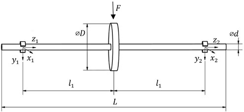
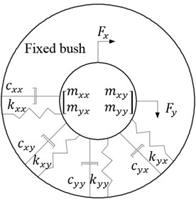
The equation of motion for a single bearing (for the model shown in Fig. 1(b)) can be described by Eq. (5). This equation can be written in the matrix form Eq. (6). The system described in this way behaves differently when it is excited in the $X$ and $Y$ direction, using the exciting force respectively $F_{X}$ and $F_{Y}$ . The system response in the $X$ direction after the excitation in the $Y$ direction is described by $X_{Y}$ :

5

{- m}_{x x} ω^{2} X_{x} {- m}_{x y} ω^{2} X_{y} + k_{x x} X_{x} + c_{x x} j ω X_{x} + k_{x y} X_{y} + c_{x y} j ω X_{y} = F_{x},

{- m}_{y y} ω^{2} Y_{y} {- m}_{x y} ω^{2} Y_{x} + k_{y y} Y_{y} + c_{y y} j ω Y_{y} + k_{y x} Y_{x} + c_{y x} j ω Y_{x} = F_{y},

6

[\begin{matrix} k_{x x} - m_{x x} ω^{2} + c_{x x} j ω & k_{x y} - m_{x y} ω^{2} + c_{x y} j ω \\ k_{y x} - m_{y x} ω^{2} + c_{y x} j ω & k_{y y} - m_{y y} ω^{2} + c_{y y} j ω \end{matrix}] [\begin{matrix} X_{x} & X_{y} \\ Y_{x} & Y_{y} \end{matrix}] = [\begin{matrix} F_{x} & 0 \\ 0 & F_{y} \end{matrix}] .

Fig. 1a) Rotor model prepared in the Samcef Rotors, b) model of one of the bearings

a)

b)

The first part of Eq. (6) is defined as the impedance and can be divided into mass, stiffness and damping parameters Eq. (7):

7

[\begin{matrix} k_{x x} - m_{x x} ω^{2} + c_{x x} j ω & k_{x y} - m_{x y} ω^{2} + c_{x y} j ω \\ k_{y x} - m_{y x} ω^{2} + c_{y x} j ω & k_{y y} - m_{y y} ω^{2} + c_{y y} j ω \end{matrix}] [\begin{matrix} 1 & 0 & {- ω}^{2} & 0 & j ω & 0 \\ 0 & 1 & 0 & {- ω}^{2} & 0 & j ω \end{matrix}]

= [\begin{matrix} k_{x x} & k_{x y} \\ k_{y x} & k_{y y} \\ m_{x x} & m_{x y} \\ m_{y x} & m_{y y} \\ c_{x x} & c_{x y} \\ c_{y x} & c_{y y} \end{matrix}] .

The least squares method is used to solve the equations and it requires the use of a signal in the frequency domain. This is achieved by Fourier transform of the force signal and the system response from the time domain. Vector $D$ is the response signal in the frequency domain, the $F$ matrix consists of the exciting force components ( $F_{x} (t)$ and $F_{y} (t)$ ) in the frequency domain. Taking into account the matrix $D$ and $F$ , Eq. (6) can be represented as Eq. (8). If we consider a system with two bearings (shown in Fig. 1(b)) the Eq. (8) can be defined as Eq. (9). Extension of a mathematical description for the system with two bearings (model shown in Fig. 1(a)) is represented by Eqs. (9)-(15):

8

[\begin{matrix} H_{{x x}_{i}} & H_{{x y}_{i}} \\ H_{{y x}_{i}} & H_{{y y}_{i}} \end{matrix}] [\begin{matrix} D_{{x x}_{i}} & D_{{x y}_{i}} \\ D_{{y x}_{i}} & D_{{y y}_{i}} \end{matrix}] = [\begin{matrix} F_{x_{i}} & 0 \\ 0 & F_{y_{i}} \end{matrix}] .

Indexes ‘1’ and ‘2’ in Eq. (9) stand for the first and the second bearing. The index ‘ $i$ ’ designates frequency range. The first of double index indicates the direction of the system response, the second index indicates the direction of the excitation force. For example, $D_{y x}^{1}$ element defines the vibrations of the rotor at the first bearing in the $x$ -direction after excitation in the $Y$ direction:

9

[\begin{matrix} H_{{x x}_{i}}^{1} & H_{{x y}_{i}}^{1} \\ H_{{y x}_{i}}^{1} & H_{{y y}_{i}}^{1} \end{matrix}] = [\begin{matrix} F_{x_{i}}^{1} & 0 \\ 0 & F_{y_{i}}^{1} \end{matrix}] {[\begin{matrix} D_{{x x}_{i}}^{1} & D_{{x x}_{i}}^{1} \\ D_{{x x}_{i}}^{1} & D_{{x x}_{i}}^{1} \end{matrix}]}^{- 1}, [\begin{matrix} H_{{x x}_{i}}^{2} & H_{{x y}_{i}}^{2} \\ H_{{y x}_{i}}^{2} & H_{{y y}_{i}}^{1} \end{matrix}] = [\begin{matrix} F_{x_{i}}^{2} & 0 \\ 0 & F_{y_{i}}^{2} \end{matrix}] {[\begin{matrix} D_{{x x}_{i}}^{2} & D_{{x x}_{i}}^{2} \\ D_{{x x}_{i}}^{2} & D_{{x x}_{i}}^{2} \end{matrix}]}^{- 1}

Flexibility is defined as the inverse of the mechanical impedance and it is presented in Eq. (10):

10

{F^{1}}_{i} = [\begin{matrix} F_{{x x}_{i}}^{1} & F_{{x y}_{i}}^{1} \\ F_{{y x}_{i}}^{1} & F_{{y y}_{i}}^{1} \end{matrix}] = {[\begin{matrix} H_{{x x}_{i}}^{1} & H_{{x y}_{i}}^{1} \\ H_{{y x}_{i}}^{1} & H_{{y y}_{i}}^{1} \end{matrix}]}^{- 1}, {F^{2}}_{i} = [\begin{matrix} F_{{x x}_{i}}^{2} & F_{{x y}_{i}}^{2} \\ F_{{y x}_{i}}^{2} & F_{{y y}_{i}}^{2} \end{matrix}] = {[\begin{matrix} H_{{x x}_{i}}^{2} & H_{{x y}_{i}}^{2} \\ H_{{y x}_{i}}^{2} & H_{{y y}_{i}}^{2} \end{matrix}]}^{- 1} .

The least squares method can be applied to the Eq. (10), it is then necessary to formulate Eq. (11). The values of matrix $Z$ can be determined from Eq. (12). In this equation, $A_{i}$ is a matrix in which the signals are elements of flexibility matrix and frequency vector. It was formed by decomposition of real and imaginary part Eq. (13). Matrix $I$ is defined by Eq. (14), while the matrix $Z$ consists of the stiffness, damping and mass coefficients of the rotor – bearings system. If we assume that the parameters are obtained for 100 frequency samples (it is determined by the index $i$ ) the matrix $A$ will have the dimensions of 800×12, matrix $I$ will have the dimensions of 800×2, while the matrix $Z$ will have dimensions of 2×12:

11

A_{i} \cdot Z = I_{i},

12

Z = {({A_{i}}^{T} A_{i})}^{- 1} {A_{i}}^{T} I_{i},

13

A_{i} = [\begin{matrix} \begin{matrix} R e a l [\begin{matrix} F_{i}^{1} & \cdot [\begin{matrix} 1 & 0 & 0 & 0 & {- (ω_{i})}^{2} & 0 & 0 & 0 & ω_{i} & 0 & 0 & 0 \\ 0 & 1 & 0 & 0 & 0 & {- (ω_{i})}^{2} & 0 & 0 & 0 & ω_{i} & 0 & 0 \end{matrix}] \end{matrix}] \\ R e a l [\begin{matrix} F_{i}^{2} & \cdot [\begin{matrix} 0 & 0 & 1 & 0 & 0 & 0 & {- (ω_{i})}^{2} & 0 & 0 & 0 & ω_{i} & 0 \\ 0 & 0 & 0 & 1 & 0 & 0 & 0 & {- (ω_{i})}^{2} & 0 & 0 & 0 & ω_{i} \end{matrix}] \end{matrix}] \end{matrix} \\ \begin{matrix} I m a g [\begin{matrix} F_{i}^{1} & \cdot [\begin{matrix} 1 & 0 & 0 & 0 & {- (ω_{i})}^{2} & 0 & 0 & 0 & ω_{i} & 0 & 0 & 0 \\ 0 & 1 & 0 & 0 & 0 & {- (ω_{i})}^{2} & 0 & 0 & 0 & ω_{i} & 0 & 0 \end{matrix}] \end{matrix}] \\ I m a g [\begin{matrix} F_{i}^{2} & \cdot [\begin{matrix} 0 & 0 & 1 & 0 & 0 & 0 & {- (ω_{i})}^{2} & 0 & 0 & 0 & ω_{i} & 0 \\ 0 & 0 & 0 & 1 & 0 & 0 & 0 & {- (ω_{i})}^{2} & 0 & 0 & 0 & ω_{i} \end{matrix}] \end{matrix}] \end{matrix} \end{matrix}],

14

I_{i} = {[\begin{matrix} 1 & 0 & 1 & 0 & 0 & 0 & 0 & 0 \\ 0 & 1 & 0 & 1 & 0 & 0 & 0 & 0 \end{matrix}]}^{T} .

The order of mass, stiffness and damping coefficients in the rotor – bearing system is shown below Eq. (15):

15

Z = {⌊\begin{matrix} k_{x x}^{1} & k_{x y}^{1} & k_{x y}^{2} \\ k_{y x}^{1} & k_{y y}^{1} & k_{y x}^{2} \end{matrix} \begin{matrix} k_{x y}^{2} & m_{x x}^{1} & m_{x y}^{1} \\ k_{y y}^{2} & m_{y x}^{1} & m_{y y}^{1} \end{matrix} \begin{matrix} m_{x x}^{2} & m_{x y}^{2} & c_{x x}^{1} \\ m_{y x}^{2} & m_{y y}^{2} & c_{y x}^{1} \end{matrix} \begin{matrix} c_{x y}^{1} & c_{x x}^{2} & c_{x y}^{2} \\ c_{y y}^{1} & c_{y x}^{2} & c_{y y}^{2} \end{matrix}⌋}^{T} .

3. Numerical model and validation

In order to verify the proposed method a numerical model of the rotor in the Samcef Rotors software was created (Fig. 1(a)). The model consists of a shaft rotating at 8 000 rpm and bearings modeled using the stiffness and damping coefficients in the orthogonal and cross-coupling directions. The rotor during the simulation had been excited by a known value of excitation force, in the central part, in the $X$ direction. Then the vibration amplitude of the rotor was measured in the each bearing in $X$ and $Y$ direction. Then, the simulation was repeated, this time using the same exciting force, but model has been excited in the $Y$ direction. In this case, the vibration amplitude of the rotor in the bearings in the direction of $X$ and $Y$ were measured. When the vibration in the $X$ direction in the first bearing after excitation in the $Y$ direction was measured, signal has been described as 1 $X_{Y}$ . Based on the excitation signals and the response signal generated by the Samcef Rotors program the stiffness, damping and mass coefficients of the bearings were calculated. Because the stiffness and damping coefficients were defined in the Samcef Rotors program it allows to compare coefficients calculated by using the proposed algorithm and the actual values.

Symmetric model of the rotor was created (Fig. 1(a)), its length is $L =$ 0.92 m. Spacing between the bearings is 2 $l_{1} =$ 0.58 m. The diameter of the rotor shaft is $d =$ 19.05 mm. At the center of the rotor is a disc having a diameter $D =$ 152.4 mm. The material of the rotor is steel with Young’s modulus of 205·10⁹ Pa, Poisson’s ratio is 0.3, the material density is 7800 kg/m³. The assumed values of the bearing stiffness and damping parameters in the main directions $x x$ , $y y$ and the cross-coupling directions $x y$ , $y x$ are shown in Tables 1 and 2. This is the standard procedure of numerical modeling of bearing-shaft systems.

Fig. 2Data processing diagram

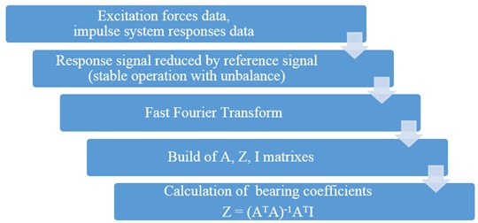
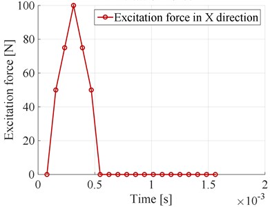
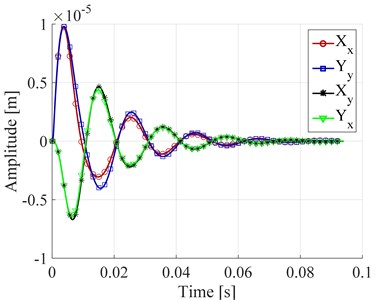
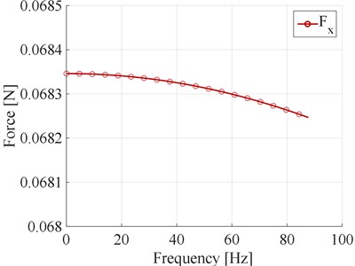
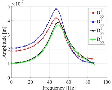
In response signal there is part connected with unbalance that cause a constant component of vibration. In practice we need to extract that component from our response signal. Data processing diagram showing whole procedure is shown in Fig. 2. In the numerical model, while the rotor was rotating it was excited by known force $F$ in the direction $X$ and the direction $Y$ respectively. The force signal in the $X$ direction is shown in Fig. 3(a). The same excitation method needs to be used in the experimental studies. Then the vibration amplitudes in the bearings were measured. Amplitude of the first bearing is shown in Fig. 3(b). Because in the described algorithm for determining the stiffness, damping and mass coefficients of rotor – bearing system signal in the frequency domain is used, it is necessary to perform a Fast Fourier Transform (FFT) of the signals. Excitation and displacement in the first bearing signal in the frequency domain are shown in Fig. 4. The function shown on the graph corresponds to the signal of the full identification range (0-87.5 Hz).

Fig. 3a) Force in the X direction as a function of time, b) displacement in the bearing number 1 as a function of time

a)

b)

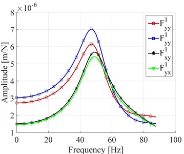
The results of a) the amplitude, b) the phase of flexibility are shown on Fig. 5. Flexibility signals are used in the described algorithm for calculating the stiffness, damping and mass coefficients of the rotor – bearing system. The resonance, visible on the graph occurs around 46 Hz and corresponding to the eigenfrequency of the described rotor. The mode shape of the rotor is shown in Fig. 6.

Fig. 4a) Force in frequency domain, b) displacement in the bearing number 1 in frequency domain

a)

b)

Fig. 5a) The flexibility of the first bearing – amplitude, b) the flexibility of the first bearing – phase

a)

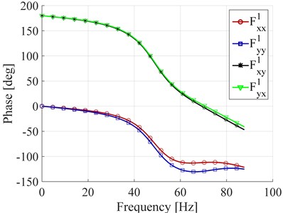
b)

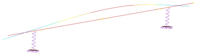
Fig. 6The first mode shape of the rotor at 46 Hz

4. Results

The signals generated using Samcef rotor program were used to calculate the stiffness, damping and mass coefficients of the rotor – bearing system. The model of symmetric rotor was considered, but the stiffness and damping coefficients (including cross-coupling values) have different values. In the hydrodynamic bearings, the cross-coupling part of damping coefficients $C_{x y}$ and $C_{y x}$ has got the same values [10], in this case they are different values in order to show how the proposed method works. Since the values of stiffness and damping coefficients were known from the numerical model, it was possible to directly compare them and on that basis it was possible to estimate an error of calculation of bearing force coefficients. The results of calculated stiffness, damping and mass coefficients are shown for two identification ranges. First of them is from 0 Hz to 3.1250 Hz, which corresponds to the value of the first three frequencies. The second identification range is from 0 Hz to 87.5 Hz, in this range the first 57 values of frequency were included. The second identification range included in the whole resonance range. Two different identification ranges were considered, because in a theoretic example only a small fragment of frequencies is sufficient. In experimental practice, researchers suggest taking into account the entire frequency range in which the resonances occur [7], this procedure enables to receive reproducible results. The results of stiffness coefficients calculation are shown in Table 1, the damping coefficients in Table 2, while the mass coefficients in Table 3.

The relative estimation error for the bearing stiffness coefficients in the first identification range does not exceed 0.02 %.The relative estimation error for the bearing stiffness coefficients in the second identification range – on the longer frequency range does not exceed 0.5 %. This is a quite accurate estimation of the stiffness coefficients of the bearings, especially given the fact that the error of calculating the stiffness coefficients within a second identification range in the main coordinates (which are more significant in further modeling of the dynamics of the system) does not exceed 0.04 %.

Table 1The stiffness coefficients

	$k_{x x}^{1}$	$k_{y y}^{1}$	$k_{x y}^{1}$	$k_{y x}^{1}$	$k_{x x}^{2}$	$k_{y y}^{2}$	$k_{x y}^{2}$	$k_{y x}^{2}$
Actual values N/m	500 000	450 000	250 000	240 000	550 000	470 000	270 000	260 000
Calculated values N/m Identification range 0-3.125 Hz	499 913	449 922	249 957	239 959	549 905	469 919	269 953	259 955
Relative error % Identification range 0-3.125 Hz	0.02	0.02	0.02	0.02	0.02	0.02	0.02	0.02
Calculated values N/m Identification range 0-87.5 Hz	499 949	449 999	249 630	241 198	550 192	469 822	270 271	259 138
Relative error % Identification range 0-87.5 Hz	0.01	0.00	0.15	0.50	0.03	0.04	0.10	0.33

The error resulting from the calculation of damping coefficients is small and in the first calculation range does not exceed 0.4 %. This error appears only in the calculation of the cross-coupling part of damping coefficients. The error of calculating the damping coefficients in second identification range is up to about 2 %.

Table 2Damping coefficients

	$c_{x x}^{1}$	$c_{y y}^{1}$	$c_{x y}^{1}$	$c_{y x}^{1}$	$c_{x x}^{2}$	$c_{y y}^{2}$	$c_{x y}^{2}$	$c_{y x}^{2}$
Actual values N/m	500	550	250	260	550	560	260	270
Calculated values N/(m/s) Identification range 0-3.125 Hz	500	550	250	259	550	560	260	271
Relative error % Identification range 0-3.125 Hz	0.00	0.00	0.00	0.38	0.00	0.00	0.00	0.37
Calculated values N/(m/s) Identification range 0-87.5 Hz	490	545	248	260	562	565	262	270
Relative error % Identification range 0-87.5 Hz	2.00	0.91	0.80	0.00	2.18	0.89	0.77	0.00

The weight of the shaft modeled in Samcef Rotors program is 4.845 kg. The calculated weight of the shaft based on described algorithm (and numerical model of the shaft) for the first identification range is 4.851 kg and for the second identification range is 4.855 kg. This mass was calculated by adding the mass coefficients on the main diagonal ( $X X$ and $Y Y$ ), and dividing this value by two. Interpretation of mass coefficient values is as follows: the mass coefficient $m_{x x}^{1}$ is the mass of part of the shaft involved with the vibration in the $X$ direction allocated to the first bearing after excitation in the $X$ direction. In contrast, the mass coefficient $m_{y y}^{1}$ is the mass of part of the shaft involved with the vibration in the $Y$ direction allocated to first bearing after excitation in the $Y$ direction. Dividing the sum of the weight coefficients by two to calculate the mass of the shaft is applied because the system was excited twice. Cross-coupling mass coefficients ( $x y$ $y x$ ) should be close to zero. The error of calculating weight coefficient for the first identification range is 0.12 % and for the second identification range 0.21 %. These results mean that the rotor weight 4.845 kg can be estimated with an accuracy of ± 0.01 kg (with the second identification range with higher relative error values).

Table 3Mass coefficients

	$m_{x x}^{1}$	$m_{y y}^{1}$	$m_{x y}^{1}$	$m_{y x}^{1}$	$m_{x x}^{2}$	$m_{y y}^{2}$	$m_{x y}^{2}$	$m_{y x}^{2}$	$\sum m$
Actual values kg									4.845
Calculated values kg Identification range 0-3.125 Hz	2.35	2.4	–0.02	0.01	2.51	2.45	0.02	–0.01	4.851
The relative error % Identification range 0-3.125 Hz									0.12
Calculated values kg Identification range 0-87.5 Hz	2.33	2.40	–0.02	0.04	2.54	2.45	0.02	–0.03	4.855
The relative error % Identification range 0-87.5 Hz									0.21

During the verification process of described algorithm used to calculate bearing force coefficients two identification ranges were checked. First identification range included only the first three frequencies from the frequency range, second included whole range in which the resonances occurred. When you expand the identification range an error increases slightly in most cases, but it is still at a relatively low level. The extension of the identification range entails less impact of the additional factors on the calculated values of mass, stiffness and damping coefficients. The author suggests that in the case of calculating one bearing (such calculations are often performed taking into account the excitation placed closely to bearing) one should apply a narrow identification range preferably from the initial frequency range.

5. Closing remarks

In the article the author extended a method for the estimation of 16 stiffness and damping coefficients of hydrodynamic bearings which was proposed by Qiu and Tieu and estimated further 8 mass coefficients. All force coefficients are calculated during a single operation using the least squares method. The calculated mass coefficients correspond to the weight of the rotor participating in the vibration of the bearings.

In order to validate the described method, the numerical model of rotor was build. Based on the known values of the exciting force and response of the system in each bearing location, stiffness, damping and mass coefficients of the rotor – bearing system were calculated.

During the work, two identification ranges were compared. The first identification range included only the range of the initial frequencies, the second identification range covered the whole resonance range. It turns out that when increasing the identification range an error increases slightly, but it is still acceptable. Extending the identification range on resonance frequencies may ensure a good reproducibility of the results in the experimental research.

References

Kiciński J. Theory and Experimental Research on Journal Slide Bearings. Flow Equipment – Maszyny Przepływowe, Wrocław, Poland, 1994, (in Polish).

Search CrossRef
Kiciński J., Żywica G. Steam Microturbines in Distributed Cogeneration. Springer Monography, 2014.

Search CrossRef
Kiciński J. Dynamics of Rotors and Slide Bearings. Flow Equipment – Maszyny Przepływowe, Gdańsk, 2005, (in Polish).

Search CrossRef
Hamrock B. J. Fundamentals of Fluid Film Lubrication. The Ohio State University, Columbus, Ohio, 1994.

Search CrossRef
Fertis D. G. Nonlinear Structural Engineering with Unique Theories and Methods to Solve Effectively Complex Nonlinear Problems. Springer, Berlin, 2010.

Search CrossRef
Nordman R., Schollhorn K. Identification of stiffness and damping coefficients of journal bearings by impact method. 2nd International Conference on Vibrations in Rotating Machinery, 1980, p. 231-238.

Search CrossRef
Qiu Z. L., Tieu A. K. Identification of sixteen force coefficients of two journal bearings from impulse responses. Wear, Vol. 212, 1997, p. 206-212.

Search CrossRef
Zhang Y. Y., Xie Y. B., Qiu D. M. Identification of linearized oil-film coefficients in a flexible rotor-bearing systems. International Conference of Hydrodynamic Bearing-Rotor System Dynamics, Xi’an, China, 1990, p. 93-108.

Search CrossRef
Chan S. H., White M. F. Experimental determination of dynamic characteristics of a full size gas turbine tilting – pad journal bearing by an impact test method. Modal Analysis, Modeling, Diagnostics and Control: Analytical and Experimental, ASME, Vol. 38, 1991, p. 291-298.

Search CrossRef
Tiwari R., Chakravarthy V. Simultaneous estimation of the residual unbalance and bearing dynamic parameters from the experimental data in a rotor-bearing system. Mechanism and Machine Theory, Vol. 44, 2009, p. 792-812.

Search CrossRef
Meruane V., Pascual R. Identification of nonlinear dynamic coefficients in plain journal bearings. Tribology International, Vol. 41, 2008, p. 743-754.

Search CrossRef
Miller B. A., Howard S. A. Identifying bearing rotor-dynamic coefficients using an extended Kalman filter. Tribology Transactions, Vol. 52, 2009, p. 671-679.

Search CrossRef
Kiciński J., Żywica G. The numerical analysis of the steam microturbine rotor supported on foil bearings. Advances in Vibration Engingeering, Vol. 11, Issue 2, 2012.

Search CrossRef
Yu Ping Wang, Daejong Kim Experimental identification of force coefficients of large hybrid air foil bearings. Gas Turbines Power, Vol. 136, Issue 3, 2013.

Search CrossRef
Delgado A. Experimental identification of dynamic force coefficients for a 110 MM compliantly damped hybrid gas bearing. Gas Turbines Power, Vol. 137, Issue 7, 2015.

Search CrossRef
Kozanek J., Simek J., Steinbauer P., Bilkovsky A. Identification of stiffness and damping coefficients of aerostatic journal bearing. Engineering Mechanics, Vol. 16, Issue 3, 2009, p. 209-220.

Search CrossRef
Jauregui J. C., San Andreas L., De Santiago O. Identification of bearing stiffness and damping coefficients using phase-plane diagrams. ASME TurboExpo2012: Turbine Technical Conference and Exposition, Vol. 7, 2012, p. 731-737.

Search CrossRef
Arora Vikas, van der Hoogt P. J. M., Aarts R. G. K. M., de Boer A. Identification of stiffness and damping characteristics of axial air-foil bearing. International Journal of Mechanics and Materials in Design, Vol. 7, Issue 3, 2011, p. 231-243.

Search CrossRef

About this article

Received

16 February 2015

Accepted

09 April 2015

Published

15 August 2015

SUBJECTS

Mechanical vibrations and applications

Keywords

force coefficients

mass

stiffness and damping coefficients

impulse response

journal bearing

Acknowledgements

Part of work described in this article was realized within the framework of STA-DY-WI-CO project, it is Marie Curie IAPP transfer of knowledge program. I would like to thank Mr. Bart Peeters for guiding me during my one year practice in the LMS International and for the possibility of using Samcef Rotors program. I would like also to thank Mr. Grzegorz Żywica for valuable comments and suggestions.

This is an open access article distributed under the Creative Commons Attribution License, which permits unrestricted use, distribution, and reproduction in any medium, provided the original work is properly cited.