Finite element modeling of a wind turbine blade

Sheibani, Mohammad; Akbari, Ali Akbar

Journal of Vibroengineering

Browse Journal

Submit article

Published: 15 November 2015

Check for updates

Finite element modeling of a wind turbine blade

Mohammad Sheibani¹

Ali Akbar Akbari²

^{1, 2}Department of Mechanical Engineering, Ferdowsi University of Mashhad, Mashhad, Iran

Corresponding Author:

Ali Akbar Akbari

Cite the article Download PDF

Downloads 1764

Abstract

Wind energy is a sustainable source of power that has a much lower environmental impact than conventional energy sources. One of the important stages in developing the modern wind turbines is studying the dynamic behavior of the flexible blades. In this article, a finite element beam model of a 150 kW horizontal axis wind turbine blade is presented. The beam elements of the present model are linear with 14 DOF and arbitrary cross sections that consider rotational velocity, shear center, warping and gyroscopic effects, stiffening due to the rotation, and all the couplings. In the present model, the cross-sectional properties along each element are variable that decreases number of the needed elements, size of the model and hence the analyses running time. By using the present model, natural frequencies, mode shapes and frequency and transient responses of the blade are extracted. The modal properties are compared with another finite element beam code BModes, and with a shell finite element model of the same blade in ABAQUS. The blade frequency and transient responses in the flap and edge directions under a turbulent wind loading are also compared with ABAQUS. Furthermore, the effects of the rotational speed and pitch angle on the blade modal properties are studied.

1. Introduction

There are many articles focusing on dynamic modeling and predicting modal properties or dynamic response of the wind turbine blades and in many cases, the blades have been modeled as a beam. Different methods have been used by different authors, including assumed modes, finite element, lumped mass and analytical methods. Arrigan et al. [1] investigated flap-wise vibration control of wind turbine blades by a single degree of freedom model with assumed mode methods approach. Zhao et al. [2] presented a new multi-body modeling methodology using a cardanic joint beam element. Kallesoe [3] derived equation of motion for a rotor blade, including gravity, pitch and rotor speed effects. Dynamic analysis of horizontal axis wind turbine was carried out by Wang et al. [4] using thin walled beam theory. Lee et al. [5] presented a method for structural dynamic modeling using multi-flexible-body method. Harte et al. [6] used one DOF assumed mode method for modeling the blades, and used spring and dampers for modeling the tower flexibility. Kessentini et al. [7] developed a mathematical model of a wind turbine using Euler-Bernoulli beam approximation and investigated modal and dynamic responses of the turbine. Murtagh et al. [8] analyzed vibrations of tower and blades of a horizontal axis wind turbine subjected to rotationally sampled wind loading. Park et al. [9] employed constrained multi-body technique to derive equations of motion for a rotating wind-turbine blade. A mathematical model of the wind turbine equipped with active controllers was formulated by Staino et al. [10] using an Euler-Lagrangian approach. Hamdi et al. [11] studied analytical and numerical dynamics of a horizontal axis wind turbine blade subjected to different types of loadings by Euler’s configuration.

In all the mentioned articles and many others, a non-verified model of a wind turbine blade has been used or developed for modal or dynamic investigations. By using a wind turbine blade model with no verification the investigation results are called into question. Hence, presenting a verified and precise model can decrease the uncertainties of further investigations on the wind turbines. There are some specific codes for dynamic analysis of wind turbines like FAST, Bladed, Flex5 and DHAT [12]. The mentioned codes, need the modal data to create a multi DOF model using the assumed-modes method. Modal data should be provided by finite element codes like BModes [13]. BModes was primarily developed by the National Renewable Energy Laboratory (NREL) to provide coupled mode shapes for FAST. This code is based on a 15 DOF beam element with three internal and two boundary nodes and is widely used. The current study aims at developing a precise model of a horizontal axis wind turbine blade with linear beam elements and 14 DOF. The beam element considers rotational velocity, shear center, warping and gyroscopic effects, stiffening due to the rotation, and all the couplings. One of the major concerns of the present study is to decrease the size of the model and hence the analysis running time without affecting the accuracy of the results by modeling the beam element with variable cross sectional properties, which is the main difference between the proposed model and other blade models and codes like BModes. Using the proposed model, a 150 kW horizontal axis wind turbine blade is modeled and the modal characteristics and the frequency and transient dynamic responses under a turbulent wind loading are extracted. Then, the modal results are compared with BModes and with a 3D model of the same blade with shell elements in ABAQUS and because the BModes cannot carry out more analysis, frequency and transient dynamic responses are only compared with ABAQUS. Furthermore, the effects of the rotational speed and pitch angle on the modal properties of the blade are studied. Because in this study, we focus on comparing the accuracy of the developed beam model with a more complicated and precise shell model in ABAQUS, the blade material is assumed to be isotropic to eliminate errors due to using equivalent composite properties provided by some codes like PreComp [14] or NuMAD [15], however, the model can consider such equivalencies. Supposing the blade is a thin walled-beam the transverse shear effect is neglected [16].

2. Blade modeling

2.1. Blade properties

General properties of the blade are presented in Table 1, and the main profiles and 3D shell model are shown in Fig. 1. Table A1 in Appendix A1 presents the properties of the blade sections made of four NREL air foils. Fig. 2 shows the normalized cross section of Airfoil S815 (the first airfoil). The shear webs are located on 20 % and 50 % of the blade chord length from the leading edge. The thickness of the blade skin and the shear webs decrease along the length of the blade. To create the airfoil splines, we have written a code in MATLAB that receives normalized coordinates of airfoils, distance to the rotor axis, chord and twist in each section and generates point coordinates to be imported to SolidWorks to create splines for the airfoils. We used ANSYS to estimate the cross-sectional properties presented in Table A2. In the table, the shear center and the centroid coordinates are with respect to the pitch center located on 25 % of the chord length (see Fig. 2), and the area moments of inertia are with respect to the centroid coordinates of each section. We assume that the pitch and shear centers are coincident and the beam cross section is rigid in its plane but is subjected to torsional warping. The coordinate system of the blade section is shown in Fig. 2. The general displacement of any arbitrary point on the blade cross section can be described as follows [17]:

1

U (x, y, z) = u - (y + e_{y}) v^{'} - (z + e_{z}) w^{'} + ψ θ^{'},

2

V (x, y, z) = v - (z + e_{z}) θ,

3

W (x, y, z) = w + (y + e_{y}) θ,

where $u$ , $v$ and $w$ , are rigid body translations of the section in the $x$ , $y$ and $z$ directions and $θ$ is the rigid body rotation about the shear center axis parallel to $x$ direction, $e_{y}$ and $e_{z}$ are the coordinates of the shear center and $ψ$ is the warping function normalized with respect to the shear center.

Fig. 1Wind turbine blade sections

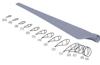
Fig. 2The blade cross section and the coordinate system

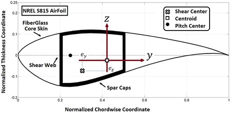
Table 1General properties of the blade

Property	Value
Material	Fiber-glass
Length	11.5 m
Density	1800 kg/m³
Mass	406 kg
Center of mass from root	4.03 m
Modulus of elasticity	18 GPa
Root joint material	Aluminum
Hub radius	0.3 m
Root joint mass	45.22 kg

2.2. The strain energy

Longitudinal strain is given by:

4

ε_{x} = \frac{\partial U}{\partial x} + \frac{1}{2} {(\frac{\partial V}{\partial x})}^{2} + \frac{1}{2} {(\frac{\partial W}{\partial x})}^{2} .

Substituting Eqs. (1)-(3) into (4), the strain function is derived as follows:

5

ε_{x} = u_{}^{'} - (y + e_{y}) v^{''} - (z + e_{z}) w^{''} + ψ θ^{''} - e_{y}^{'} v^{'} - e_{z}^{'} w^{'}

+ 0.5 {(v^{'} - (z + e_{z}) θ^{'} - e_{z}^{'} θ)}^{2} + 0.5 {(w^{'} + (y + e_{y}) θ^{'} + e_{y}^{'} θ)}^{2} .

Because displacement in $x$ direction ( $u$ ) is dependent on $v$ and $w$ , a new variable ( $s$ ) which is the arc length stretch of the element is defined as follows:

6

s^{'} = ε_{x} (- e_{y}, - e_{z}) = u_{}^{'} - e_{y}^{'} v^{'} - e_{z}^{'} w^{'} + 0.5 {(v^{'} - e_{z}^{'} θ)}^{2} + 0.5 {(w^{'} + e_{y}^{'} θ)}^{2},

thus:

7

u_{}^{'} = s^{'} + e_{y}^{'} v^{'} + e_{z}^{'} w^{'} - 0.5 {(v^{'} - e_{z}^{'} θ)}^{2} - 0.5 {(w^{'} + e_{y}^{'} θ)}^{2},

8

u_{} = s + \int_{0}^{x} [e_{y}^{'} v^{'} + e_{z}^{'} w^{'} - 0.5 {(v^{'} - e_{z}^{'} θ)}^{2} - 0.5 {(w^{'} + e_{y}^{'} θ)}^{2}] d η .

After some manipulation $u$ has the form:

9

u_{} = s + e_{y} v^{'} + e_{z} w^{'} + D (x, t),

where:

10

D (x, t) = \int_{0}^{x} [e_{y} v^{''} + e_{z} w^{''} - 0.5 {(v^{'} - e_{z}^{'} θ)}^{2} - 0.5 {(w^{'} + e_{y}^{'} θ)}^{2}] d η .

Substituting Eq. (9) into Eq. (1), one obtains:

11

U = s - y v^{'} - z w^{'} + ψ θ^{'} + D (x) .

Substituting Eqs. (2), (3) and (9) into Eq. (4), the longitudinal strain can be written as:

12

ε_{x} = s^{'} - (y + e_{y}) v^{''} - (z + e_{z}) w^{''} + ψ θ^{''} + 0.5 {(v^{'} - (z + e_{z}) θ^{'} - e_{z}^{'} θ)}^{2}

+ 0.5 {(w^{'} + (y + e_{y}) θ^{'} + e_{y}^{'} θ)}^{2} - 0.5 {(v^{'} - e_{z}^{'} θ)}^{2} - 0.5 {(w^{'} + e_{y}^{'} θ)}^{2} .

Neglecting non-linear terms, strain along $x$ direction becomes:

13

ε_{x} = s^{'} - (y + e_{y}) v^{''} - (z + e_{z}) w^{''} + ψ θ^{''} .

Substituting Eqs. (2), (3), (11) into the shear strain equations, one obtains:

14

γ_{x y} = (\frac{\partial ψ}{\partial y} - (z + e_{z})) θ^{'} - e_{z}^{'} θ,

15

γ_{x z} = (\frac{\partial ψ}{\partial z} + (y + e_{y})) θ^{'} + e_{y}^{'} θ,

16

γ_{x z} = 0 .

The elastic strain energy is given by:

17

Π = \frac{1}{2} ∭ (E ε_{x}^{2} + G γ_{x y}^{2} + G γ_{x z}^{2}) d v,

where $E$ and $G$ are the modules of elasticity and shear modules, respectively. Substituting Eqs. (12)-(15) into Eq. (17), the potential energy is derived as follows:

18

Π = \frac{1}{2} ∭ (E {(s^{'} - (y + e_{y}) v^{''} - (z + e_{z}) w^{''} + ψ θ^{''})}^{2}

+ G {((\frac{\partial ψ}{\partial y} - (z + e_{z})) θ^{'} - e_{z}^{'} θ)}^{2} + G {((\frac{\partial ψ}{\partial z} + (y + e_{y})) θ^{'} + e_{y}^{'} θ)}^{2}) d v,

where $d v$ is the differential of the element volume. Ignoring higher orders of $e_{y}$ and $e_{z}$ and defining:

19

I_{y} = \iint z^{2} d A, I_{z} = \iint y^{2} d A, I_{y z} = \iint y z d A, Γ = \iint ψ^{2} d A,

in which $I_{y}$ , $I_{z}$ , $I_{y z}$ are the area moments of inertia and $Γ$ is the warping constant. Considering the following equalities [20]:

20

\iint ψ d A = 0, \iint y ψ d A = 0, \iint z ψ d A = 0, \iint \frac{\partial ψ}{\partial y} d A = 0, \iint \frac{\partial ψ}{\partial z} d A = 0,

and integrating over the cross section area, the potential energy can be written as:

21

Π_{t o t a l} = Π_{E . B} + Π_{S . C},

where $Π_{E . B}$ is the potential energy of an Euler-Bernoulli beam and $Π_{S . C}$ is the potential energy due to the shear center effect as follows:

22

Π_{E . B} = \frac{1}{2} \int_{0}^{l} \{E (A {s^{'}}^{2} + I_{z} {v^{''}}^{2} + I_{y} {w^{''}}^{2} + 2 I_{y z} v^{''} w^{''} + Γ {θ^{''}}^{2}) + G J^{*} {θ^{'}}^{2}\} d x,

23

Π_{S . C} = \frac{1}{2} \int_{0}^{l} E (- 2 A (e_{y} {v^{''} s}^{'} + e_{z} w^{''} s^{'}) + G J^{* *} {θ^{'}}^{2}) d x,

in which $J^{*}$ and $J^{* *}$ are the Saint-Venant’s torsion constant given by:

24

J^{*} = \iint ({(\frac{\partial ψ}{\partial y} - z)}^{2} + {(\frac{\partial ψ}{\partial z} + y)}^{2}) d A,

25

J^{* *} = 2 \iint (e_{z} \frac{\partial ψ}{\partial y} + e_{y} \frac{\partial ψ}{\partial z}) d A + A (e_{y}^{2} + e_{z}^{2}) .

2.3. The kinetic energy

Considering the rotational speed of the beam in $y$ and $z$ directions as follows:

26

\vec{Ω} = {[\begin{matrix} 0 & Ω_{y} & Ω_{z} \end{matrix}]}^{T} .

The velocity vector is given by:

27

\vec{V} = {\dot{\vec{r}}}_{p^{*}} + \vec{Ω} \times {\vec{r}}_{p^{*}},

where ${\vec{r}}_{p^{*}}$ is the new position of an arbitrary point $p$ after deflection:

28

{\vec{r}}_{p^{*}} = {[x, y, z]}^{T} + {[U, V, W]}^{T} .

Substituting Eq. (28) into Eq. (27) and using Eqs. (2), (3) and (11) one obtains:

29

\vec{V} = \{\begin{array}{l} (\begin{matrix} \dot{s} - \frac{1}{2} {\dot{D}}_{2} (x) - y {\dot{v}}_{s}^{'} - z {\dot{w}}_{s}^{'} + ψ {\dot{θ}}^{'} + {\dot{D}}_{1} \\ + Ω_{y} (z + w_{} + (y + e_{y}) θ) - Ω_{z} (y + v_{} - (z + e_{z}) θ) \end{matrix}), \\ {\dot{v}}_{} - (z + e_{z}) \dot{θ} + Ω_{z} (x + s - y v_{}^{'} - z w_{}^{'} + ψ θ^{'} + D (x)), \\ {\dot{w}}_{} + (y + e_{y}) \dot{θ} - Ω_{y} (x + s - y v_{}^{'} - z w_{}^{'} + ψ θ^{'} + D (x)), \end{array}

in which:

30

D_{1} = \int_{0}^{x} [e_{y} v^{''} + e_{z} w^{''}] d η, D_{2} = \int_{0}^{x} [{(v^{'} - e_{z}^{'} θ)}^{2} + {(w^{'} + e_{y}^{'} θ)}^{2}] d η .

The kinetic energy is given by:

31

T = \frac{1}{2} ρ ∭ \vec{V} \vec{V} d v,

where $ρ$ is density per unit volume. Substituting Eq. (29) into Eq. (31) and integrating over the cross section area and ignoring non-linear terms, the kinetic energy can be written as:

32

T_{t o t a l} = T_{E . B} + T_{w a r p} + T_{s c} + T_{r o t} + T_{s c - r o t} + T_{w a r p - r o t},

where $T_{E . B}$ is the kinetic energy of an Euler-Bernoulli beam, $T_{w a r p}$ , $T_{s c}$ and $T_{r o t}$ are the kinetic energies due to the warping and shear center effects and the rotational speed, respectively, $T_{s c - r o t}$ is the kinetic energy due to the simultaneous effects of the shear center and the rotational speed and $T_{w a r p - r o t}$ is the kinetic energy due to the simultaneous effects of the warping and rotational speed, as follows:

33

T_{E . B} = 0.5 ρ \int_{0}^{l} \{A ({\dot{s}}^{2} + {\dot{v}}^{2} + {\dot{w}}^{2}) + (I_{y} + I_{z}) {\dot{θ}}^{2} + (I_{y} {\dot{w}}^{' 2} + I_{z} {\dot{v}}^{'}^{2} + 2 I_{y z} {\dot{v}}^{'} \dot{w}')\} d x,

34

T_{r o t} = 0.5 ρ \int_{0}^{l} \{2 Ω_{y} (A (x \dot{w} + w \dot{s} - s \dot{w}) - I_{y} {\dot{w}}^{'} + I_{z} (v^{'} \dot{θ} - {\dot{v}}^{'} θ)

+ I_{y z} (w^{'} \dot{θ} - {\dot{w}}^{'} θ - {\dot{v}}^{'})) + 2 Ω_{z} (A (x \dot{v} - v \dot{s} + s \dot{v}) + I_{y} (w^{'} \dot{θ} - {\dot{w}}^{'} θ)

+ I_{z} {\dot{v}}^{'} + I_{y z} (v^{'} \dot{θ} - {\dot{v}}^{'} θ + {\dot{w}}^{'})) {+ Ω}_{y}^{2} (I_{y} + A w^{2}) + Ω_{z}^{2} (I_{z} + A v^{2})

+ (Ω_{y}^{2} + Ω_{z}^{2}) (A x^{2} + A s^{2} + 2 A x s + I_{y} {w^{'}}^{2} + I_{z} {v^{'}}^{2} + 2 I_{y z} v^{'} w^{'})

- 2 Ω_{y} Ω_{z} (I_{y z} + A w v) + 2 ((I_{y} - I_{z}) Ω_{y} Ω_{z} + I_{y z} (Ω_{y}^{2} - Ω_{z}^{2})) θ

+ (I_{z} Ω_{y}^{2} + I_{y} Ω_{z}^{2} + 2 I_{y z} Ω_{y} Ω_{z}) θ^{2}\} d x - 0.5 ρ (Ω_{y}^{2} + Ω_{z}^{2}) \int_{0}^{l} (\int_{x}^{l} A η d η) ({v^{'}}^{2} + {w^{'}}^{2}) d x,

35

T_{w a r p} = 0.5 ρ \int_{0}^{l} Γ {\dot{θ}}^{' 2} d x,

36

T_{w a r p - r o t} = 0.5 ρ \int_{0}^{l} (Ω_{y}^{2} + Ω_{z}^{2}) (Γ {θ^{'}}^{2}) d x,

37

T_{s c} = 0.5 ρ \int_{0}^{l} A \{(e_{y}^{2} + e_{z}^{2}) {\dot{θ}}^{2} + 2 (e_{y} \dot{w} \dot{θ} - e_{z} \dot{v} \dot{θ}) + 2 \dot{s} {\dot{D}}_{1} + {\dot{D}}_{1}^{2}\} d x,

38

T_{s c_{r o t}} = 0.5 ρ \int_{0}^{l} A \{{(Ω_{y} e_{y} + Ω_{z} e_{z})}^{2} θ^{2} + 2 Ω_{y} (w_{s} {\dot{D}}_{1} - {\dot{w}}_{s} D_{1}) + 2 Ω_{z} (- v_{s} {\dot{D}}_{1} + {\dot{v}}_{s} D_{1})

+ (Ω_{y}^{2} + Ω_{z}^{2}) (D_{1}^{2} + 2 x D_{1} + 2 s D_{1}) + 2 (Ω_{y} e_{y} + Ω_{z} e_{z}) (\dot{s} θ - x \dot{θ} - s \dot{θ} + Ω_{y} w θ

- Ω_{z} v θ + θ {\dot{D}}_{1} - \dot{θ} D_{1})\} d x + 0.5 ρ (Ω_{y}^{2} + Ω_{z}^{2}) \int_{0}^{l} 2 (\int_{x}^{l} A η d η) ({- e_{z}^{'} v^{'} θ + e}_{y}^{'} w^{'} θ) d x .

2.4. Finite elements discretization

In order to derive the finite element matrices, a displacement field should be assumed. The nodal vector of seven local displacement parameters is defined as:

39

q = {[s v w θ_{x} θ_{y} θ_{z} θ_{x}^{'}]}^{T},

in which:

θ_{y} = - w^{'}, θ_{z} = v^{'} .

A liner interpolation is considered for the axial displacement, and a cubic Hermitian function for the lateral deflection and torsion:

40

s = N_{s} q_{s}, v = N_{v} q_{v}, w = N_{w} q_{w}, θ = N_{θ} q_{θ},

where:

41

N_{s} = [\begin{matrix} 1 - ξ & 0 & ξ & 0 \end{matrix}], N_{v} = [\begin{matrix} f_{1} & l f_{2} & f_{3} & - l f_{4} \end{matrix}],

N_{w} = [\begin{matrix} f_{1} & - l f_{2} & f_{3} & - l f_{4} \end{matrix}], N_{θ} = {[\begin{matrix} θ_{x 1} & θ_{x 1}^{'} & \begin{matrix} θ_{x 2} & θ_{x 2}^{'} \end{matrix} \end{matrix}]}^{T},

q_{s} = {[\begin{matrix} s_{1} & θ_{x 1}^{'} & \begin{matrix} s_{2} & θ_{x 2}^{'} \end{matrix} \end{matrix}]}^{T}, q_{v} = {[\begin{matrix} v_{1} & θ_{z 1} & \begin{matrix} v_{2} & θ_{z 2} \end{matrix} \end{matrix}]}^{T},

q_{w} = {[\begin{matrix} w_{1} & θ_{y 1} & \begin{matrix} w_{2} & θ_{y 2} \end{matrix} \end{matrix}]}^{T}, q_{θ} = {[\begin{matrix} θ_{x 1} & θ_{x 1}^{'} & \begin{matrix} θ_{x 2} & θ_{x 2}^{'} \end{matrix} \end{matrix}]}^{T},

in which:

42

f_{1} = 1 - 3 ξ^{2} + 2 ξ^{3}, f_{2} = ξ - 2 ξ^{2} + ξ^{3}, f_{3} = 3 ξ^{2} - 2 ξ^{3}, f_{4} = - ξ^{2} + ξ^{3}, ξ = \frac{x}{l} .

Using the Lagrange’s equation, given by:

43

\frac{d}{d t} (\frac{\partial T}{\partial {\dot{q}}_{i}}) - \frac{\partial T}{\partial q_{i}} + \frac{\partial Π}{\partial q_{i}} = Q_{i},

and Eq. (44) the differential equation of motion can be written as follows:

44

M \ddot{q} + C^{*} \dot{q} + K q = F,

where $M$ and $K$ are the mass and stiffness matrices, $F$ is the force vector due to the blade rotational speed, and:

45

C^{*} = D + C,

in which, $C$ is the damping matrix and $D$ is a matrix due to the rotational effects. Substituting Eq. (40) into Eq. (22), (23) and Eq. (33)-(38) and using the Lagrange’s equation, all mass, stiffness and rotational effect matrices of the single and coupled DOFs are derived and presented in Appendix A2.

3. Modal analysis

After deriving the bam element matrices, we used MATLAB to write a code to compute all the matrices for the 150 kW wind turbine blade and assemble them. It should be mentioned that in the beam element model, the blade skin and the shear web thickness vary along the length of the blade, while in ABAQUS the blade is divided into 13 sections with constant thickness (see Table A1 in Appendix A1), thus the blade mass properties in ABAQUS and the code would not be the same. To solve the problem, cross-sectional properties of the MATLAB code are updated by multiplying correction coefficients. Table 2 presents the six first natural frequencies of the clamped blade computed by ABAQUS, the present model and BModes, and compares the results. Since all the modes are coupled, each mode shape includes flap, edge, longitudinal and torsional deflections. The flap and the edge directions are parallel to $z$ and $y$ axis, respectively. Longitudinal and torsional deflections are small, but the torsional deflection is more important because it changes the blade twist angle and affects the aerodynamic forces. Major deflections occur in the flap and edge directions. The blade stiffness in the flap direction is lower than the edge direction (see Table A2 in Appendix A1) so it has more contributions in the first six mode shapes. Only in the second and fifth mode shapes, edge deflection is dominant. According to the table, the predictions of the present model are in good agreement with ABAQUS and more precise than BModes. Fig. 3 shows the first six mode shapes of the blade in ABAQUS. By selecting a path of nodes along the length of the blade in ABAQUS the bending mode shapes have been extracted and depicted in Fig. 4 and compared with the mode shapes computed by the present model. The ABAQUS model has 8800 quadratic shell elements, and the current model has 13 elements. Fig. 5 compares the bending mode shapes differences of the present model and BModes with ABAQUS (BModes has 50 elements). As seen in Fig. 4 and 5, the proposed model results are in good agreement with ABAQUS and are relatively better than BModes.

Fig. 3Blade mode shapes in ABAQUS

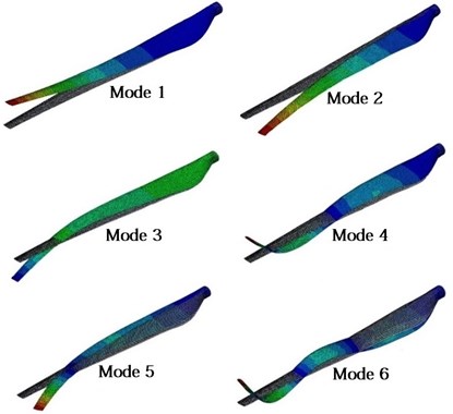
Fig. 4Blade bending mode shapes in the present model and ABAQUS

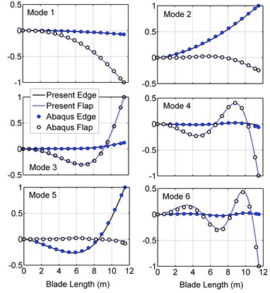
Table 2The blade natural frequencies

Mode number	Dominant mode shape	Abaqus (Hz)	Present (Hz)	Abaqus-present difference	Bmodes (Hz)	Abaqus-Bmodes difference
1	Flap 1st	2.423	2.406	–0.69 %	2.545	5.03 %
2	Edge 1st	5.887	5.910	0.39 %	5.972	1.44 %
3	Flap 2nd	7.245	7.266	0.29 %	7.735	6.77 %
4	Flap 3rd	16.23	16.31	0.46 %	17.44	7.45 %
5	Edge 2nd	20.48	20.37	–0.55 %	20.44	–0.17 %
6	Flap 4th	28.70	29.11	1.44 %	31.44	9.55 %

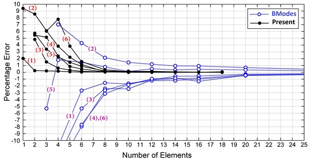
Fig. 6 shows the torsional mode shapes in BModes and the present model and the average torsion of each blade cross section in ABAQUS. In the shell model of ABAQUS, distortions of the blade surfaces make it difficult to extract the torsional mode shapes smoothly, especially because these mode shapes are very smaller than the dominant modes. Although the mode shapes are not smooth in some frequencies, differences between all three models are in an acceptable range. Fig. 7 compares the natural frequency convergence of the proposed model with BModes. As seen in the figure, the current model rapidly converges, and only seven elements are needed to decrease the percentage error of the first six frequencies to 1 % of the final values, while BModes needs more than 18 elements. Using five elements, all frequencies of the present model have less than 4 % error, and just by one element, the proposed model can predict the first natural frequency with 2 % error, which is very useful for studies that the first flap vibrations are only considered [1, 4, 7]. As a conclusion, for a very small number of elements, the current model is much more accurate than BModes.

3.1. Effect of the rotational speed on the natural frequencies

Due to the rotational effects, the blade natural frequencies depend on the rotor speed. By increasing the rotational speed, the blade stiffness and hence the natural frequencies increase. Eqs. (A19)-(A33) (see Appendix A2) present stiffness matrices due to the rotational speed, where $θ$ is the pitch angle (angle between the rotation axis and $z$ axis). Eq. (A19)-(A23) (see Appendix A2) are only related to the rotational speed, while Eq. (A24) (see Appendix A2) is related to the simultaneous effect of the rotational speed and the warping, and Eq. (A25)-(A33) (see Appendix A2) are presenting the simultaneous effects of the rotation and the shear center.

Fig. 5Bending mode shapes differences of the present model and BModes compared with ABAQUS

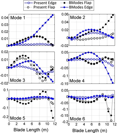
Fig. 6Blade torsional mode shapes in the present model, BModes and ABAQUS

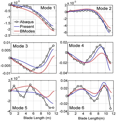
Fig. 7Natural frequencies convergence for the present model and BModes

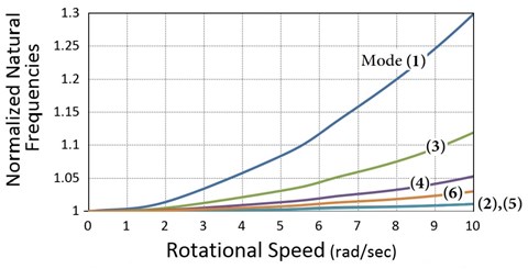
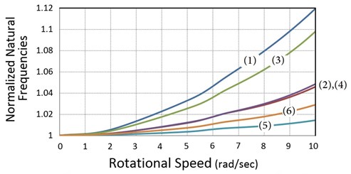
The blade normalized frequencies versus the rotational speed at zero and 90° pitch angle are presented in Fig. 8. Here the distance between the rotation axis and the first section of the blade (hub radius) is 0.3 m. As seen in the figure, angular velocity has a considerable impact on the natural frequencies. At the nominal rotor speed (6.28 r/s) and zero pitch angle (Fig. 8(a)), natural frequency of the first mode increases about 12 %. The figure shows that the dominant flap frequencies increase more than the dominant edge frequencies which can be described by Eq. (A22) (see Appendix A2) that is the flap stiffness due to the rotational speed. At zero pitch angle ( $θ = 0$ ), the second term of the equation becomes zero, while in Eq. (A20) which is the rotational stiffness in the edge direction, the second term has its maximum value, so stiffness in the flap direction has its maximum value while stiffness in the edge direction has its minimum value, hence the flap frequencies are more sensitive to the speed changes. In Eqs. (A20), (A22), (see Appendix A2) $I_{z}$ and $I_{y}$ are negligible in comparison with:

46

\int_{x}^{l} A η d η .

By increasing the pitch angle, frequencies are less sensitive to the rotational speed and as seen in Fig. 8(b), at nominal rotor speed and 90° pitch angle the first frequency increases about 5 %. Because the area moment of inertia and hence the stiffness in the edge direction is on average 10 times bigger than inertia in the flap direction, the same increase in the edge and flap stiffness would have less effect on the edge frequencies. Consequently, in Fig. 8(b), again the flap frequencies increase more than the edge frequencies, while in Eq. (A20) (see Appendix A2) the second term has its maximum value. Table 3 presents the percentage differences of the model results comparing with ABAQUS. According to the table, except for the sixth mode all differences are less than 1 %.

Fig. 8Rotor speed effect on the natural frequencies

a) Zero pitch angle

b) 90° pitch angle

Table 3Percentage differences of the present model natural frequencies compared with ABAQUS at four rotational velocities

Mode number	90° pitch angle				Zero pitch angle
Mode number	2 (r/s)	5 (r/s)	6.28 (r/s)	10 (r/s)	2 (r/s)	5 (r/s)	6.28 (r/s)	10 (r/s)
1	0.66 %	0.57 %	0.50 %	0.33 %	0.68 %	0.64 %	0.59 %	0.53 %
2	0.40 %	0.42 %	0.56 %	0.53 %	0.39 %	0.42 %	0.55 %	0.52 %
3	0.29 %	0.29 %	0.30 %	0.29 %	0.29 %	0.29 %	0.30 %	0.30 %
4	0.42 %	0.45 %	0.47 %	0.41 %	0.44 %	0.44 %	0.47 %	0.43 %
5	0.55 %	0.52 %	0.49 %	0.49 %	0.56 %	–0.55 %	0.45 %	0.49 %
6	1.46 %	1.43 %	1.50 %	1.42 %	1.46 %	1.43 %	1.49 %	1.43 %

3.2. Effect of the rotational speed on the mode shapes

The blade mode shapes are also affected by the rotational speed. The first three mode shapes in three different rotational speeds and zero pitch angle are shown in Fig. 9. According to the figure, rotational speeds up to 10 r/s have no impact on dominant mode shapes, but non-dominant mode shapes are slightly affected.

Fig. 9Blade mode shapes of the present model at different rotational speeds

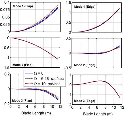
Fig. 10Percentage changes of the blade natural frequencies (Ω= 6.28 rad/sec)

3.3. Effect of the pitch angle

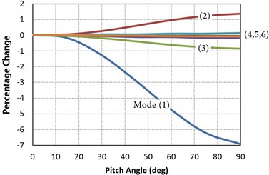
In pitch control wind turbines, the blade pitch angle varies with the wind speed and the rotational velocity that affects the natural frequencies of the blade and the turbine as well. Fig. 10 illustrates percentage changes of the blade natural frequencies from zero to 90° pitch angle at the nominal rotor speed. According to the figure, the lower mode shapes are more affected by changing the blade pitch angle. At maximum practical pitch angle (30°), the first frequency has the most reduction by about 1.2 %. Thus, the effect of the pitch angle on the natural frequencies in practical pitch angles is negligible. Eqs. (A20), (A22) (see Appendix A2) describe why the flap dominant frequencies (modes 1, 3, 4 and 6) decrease while the edge dominant frequencies (modes 2 and 5) increase. By increasing the pitch angle, the second term of Eq. (A20) (see Appendix A2) decreases, hence the stiffness of the edge direction increases, while the second term of Eq. (A22) (see Appendix A2) increases and hence the stiffness of the flap direction decreases. Table 4 presents the percentage differences between the present model and ABAQUS results which are in an acceptable range.

Table 4Percentage differences of the present model natural frequencies at 6.28 r/s

Mode number	Pitch angle
Mode number	15°	30°	45°	60°	75°
1	0.26 %	0.11 %	0.07 %	0.15 %	0.35 %
2	0.52 %	0.49 %	0.48 %	0.48 %	0.52 %
3	0.32 %	0.33 %	0.33 %	0.33 %	0.33 %
4	0.48 %	0.48 %	0.42 %	0.48 %	0.48 %
5	0.49 %	0.48 %	0.48 %	0.49 %	0.49 %
6	1.52 %	1.48 %	1.48 %	1.48 %	1.48 %

4. Frequency and transient response

Blade tip deflection is an important consideration in the wind turbine design process. If the blade deflects too much, significant stress are applied to the blade, and also the blade may hit the tower. Here we investigate the frequency and transient response of the blade tip by considering the damping matrix as follows [19]:

47

C = M (\sum_{n = 1}^{N} \frac{2 ξ_{n} ω_{n}}{M_{n}} ϕ_{n} ϕ_{n}^{T}) M,

where $M$ and $C$ are mass and damping matrices, $ξ_{n}$ , $ω_{n}$ , $M_{n}$ and $ϕ_{n}$ are damping ratio, natural frequency, modal mass and mode shape of mode $n$ , respectively. Here the damping ratio is considered to be 1 % for the first 10 modes.

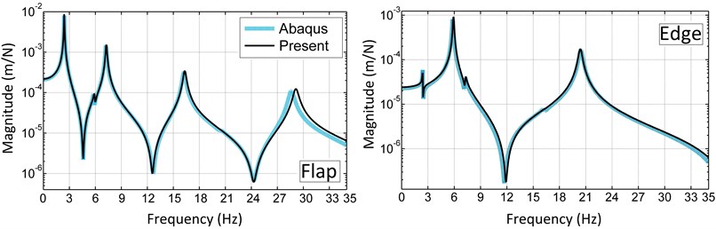
Point FRFs of the blade tip for the flap and edge directions in zero rotational speed and zero pitch angle are presented in Fig. 11. In the flap FRF, the first edge frequency is observable and in the edge FRF the first two flap frequencies are visible. As seen in the figure, there is good agreement between the results of the present model and ABAQUS.

Fig. 11The blade tip point FRFs in the flap and edge directions

One of the important loads acting on the blade is a periodic force due to the blade rotation and the wind shear. In this section, the transient response of the blade tip under a turbulent wind load is investigated. The drag force per unit length exerted on the blade is given by:

48

f (x, t) = 0.5 ρ L_{c} C_{d} V^{2},

where $L_{c}$ , $C_{d}$ and $V$ are the chord length, the drag coefficient and the wind speed, respectively. The wind speed function along the length of the blade is given by:

49

V (x, t) = V_{h u b} + V_{h u b} ({(1 + \frac{x}{H_{h u b}})}^{α} - 1) \sin (Ω t),

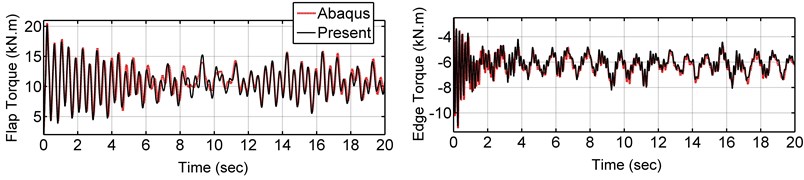
where $H_{h u b}$ , and $V_{h u b}$ are the hub height and wind speed at the hub height, $x$ is the blade length variable, $α$ is the wind shear exponent and $Ω$ is the blade rotational speed. Table 5 presents the constant values of Eq. (48)-(49). Fig. 12 shows the turbulent wind speed for 20 seconds at the hub height taken from Binalood Wind farm in Iran [20], and the wind speed at the blade tip height (hub height plus the blade length) due to the wind shear and the rotor speed. The wind force is applied to the model at three nodes. The resultant force from the first element to element 5 is applied at node 4, resultant force from element 6 to element 9 is applied at node 8 and resultant force from element 9 to element 13 is applied at node 12. Fig. 13 shows these three resultant forces resulted from Eq. (48). The time response of the blade tip deflection for 30° of pitch angle is shown in Fig. 14. Fig. 15 and 16 present reaction forces and torques of the blade root joint in the flap and edge directions. As seen in the figure, the current model accurately predicts the blade tip displacements and the root forces and torques under the turbulent wind loading.

Table 5Constant values of Eqs. (48)-(49)

$ρ$	$C_{d}$	$H_{h u b}$	$α$	$Ω$ (r/s)
1.05 kg/m³	1.2	36 m	0.2034	6.28

Fig. 12Wind speed at the hub height and blade tip

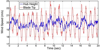
Fig. 13Wind loads applying on the blade

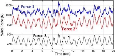
Fig. 14Blade tip displacement in the flap and edge directions at 30° pitch angle

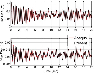
Fig. 15Reaction forces of the blade root joint in the flap and edge directions at 30° pitch angle

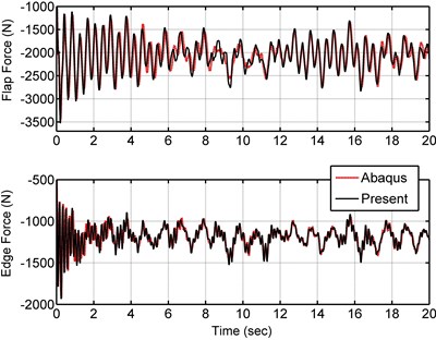
Fig. 16Reaction torques of the blade root joint in the flap and edge directions at 30o pitch angle

5. Conclusions

In the current study, a blade beam finite element model with 14 degrees of freedom and arbitrary cross section which considers rotational velocity, shear center, warping and gyroscopic effects, stiffening due to the rotation, and all the couplings has been developed to model a 150 kW horizontal axis wind turbine blade. In the present model, number of the needed blade elements has been significantly decreased by using the elements with variable cross sectional properties. The modal result and frequency convergence of the model was compared with BModes, and the modal, frequency and transient responses compared with a shell finite element model in ABAQUS. Moreover, the effects of the rotational speed and pitch angle on the natural frequencies and the mode shapes were investigated, and the results compared with ABAQUS. According to the results, the present model has accurately predicted the natural frequencies and the mode shapes. In addition, it was shown that by using just seven elements, the percentage error of the present model for the first six natural frequencies decreased to 1 %, while another widely used finite element code, BModes needed more than 18 elements for the same result. For a very small number of elements, the present model predictions were much better than BModes, and using only one element the first natural frequency had only 2 % error. It was seen that the rotational velocity affected the first frequency more than other modes and increased it about 12 % at the nominal rotor speed and zero pitch angle. Dominant mode shapes were not sensitive to the rotational speed, while the non-dominant mode shapes were slightly affected. The pitch angle had a small effect on the natural frequencies. By increasing the pitch angle, the first natural frequency decreased about 1.2 % at the nominal rotor speed and 30° of pitch angle. At the next step, point FRFs of the blade tip for the edge and the flap directions presented. It was shown that the first, third, fourth and sixth modes in the flap FRF and the second and fifth modes in the edge FRF were dominant. Then, the transient response of the blade tip deflections and the blade root joint reaction forces and torques under a turbulent wind load for 30° pitch angle were depicted. Comparing the modal, frequency and transient results of the model with BModes and ABAQUS, it was shown that the current model had accurate predictions with less computational cost. Hence, the present beam model can be a proper alternative for more detailed and complicated 3D models, especially to facilitate the blade structural design and optimization process in the preliminary design stages, and can decrease the analyses running time without affecting the accuracy of the results. Since the model has good predictions with a very small number of elements, it also can be used instead of other simple models without a great increase in computational cost.

References

Arrigan J., Pakrashi V., Basu B., Nagarajaiah S. Control of flapwise vibrations in wind turbine blades using semi-active tuned mass dampers. Structural Control and Health Monitoring, Vol. 18, Issue 8, 2011, p. 840-851.

Search CrossRef
Xueyong Z., Maißer P., Wu J. A new multibody modelling methodology for wind turbine structures using a cardanic joint beam element. Renewable Energy, Vol. 32, Issue 3, 2007, p. 532-546.

Search CrossRef
Kallesøe B. S. Equations of motion for a rotor blade, including gravity, pitch action and rotor speed variations. Wind Energy, Vol. 10, Issue 3, 2007, p. 209-230.

Search CrossRef
Wang J., Qin D., Teik C. L. Dynamic analysis of horizontal axis wind turbine by thin-walled beam theory. Journal of Sound and Vibration, Vol. 329, Issue 17, 2010, p. 3565-3586.

Search CrossRef
Lee D., Hodges D., Patil M. Multi-flexible-body dynamic analysis of horizontal axis wind turbines. Wind Energy, Vol. 5, Issue 4, 2002, p. 281-300.

Search CrossRef
Harte M., Basu B., Nielsen S. R. Dynamic analysis of wind turbines including soil-structure interaction. Engineering Structures, Vol. 45, 2012, p. 509-518.

Search CrossRef
Kessentini S., Choura S., Najar F., Franchek M. A. Modeling and dynamics of a horizontal axis wind turbine. Journal of Vibration and Control, Vol. 16, Issue 13, 2010, p. 2001-2021.

Search CrossRef
Murtagh P. J., Basu B., Broderick B. M. Along-wind response of a wind turbine tower with blade coupling subjected to rotationally sampled wind loading. Engineering Structures, Vol. 27, Issue 8, 2005, p. 1209-219.

Search CrossRef
Park J. H., Park H. Y., Jeong S. Y., Lee S., Shin Y. H., Park J. P. Linear vibration analysis of rotating wind-turbine blade. Current Applied Physics, Vol. 10, Issue 2, 2010, p. 332-334.

Search CrossRef
Staino A., Basu B., Nielsen S. R. Actuator control of edgewise vibrations in wind turbine blades. Journal of Sound and Vibrations, Vol. 31, Issue 6, 2012, p. 1233-1256.

Search CrossRef
Hamdi H., Mrad C., Hamdi A. Nasri R. Dynamic response of a horizontal axis wind turbine blade under aerodynamic, gravity and gyroscopic effects. Applied Acoustics, Vol. 86, 2014, p. 154-164.

Search CrossRef
Ahlström A. Aeroelastic Simulation of Wind Turbine Dynamics. Dissertation, Tekniska Högskolan, Stockholm, 2005.

Search CrossRef
NWTC Information Portal (BModes). https://nwtc.nrel.gov/BModes, 2014.

Search CrossRef
NWTC Information Portal (PreComp). https://nwtc.nrel.gov/PreComp, 2014.

Search CrossRef
Berg J. C., Resor B. R. Numerical Manufacturing and DesignTool (NuMAD v2.0) for Wind Turbine Blades: User’s Guide. Sandia National Laboratories, California, USA, 2012.

Search CrossRef
Liviu L., Song O. Thin-walled Composite Beams: Theory and Application. Springer, Dordrecht, the Netherlands, 2006.

Search CrossRef
Vörös Gábor M. On coupled bending-torsional vibrations of beams with initial loads. Mechanics Research Communications, Vol. 36, Issue 5, 2009, p. 603-611.

Search CrossRef
Subrahmanyam K. B., Kulkarni S. V., Rao J. S. Application of the Reissner method to derive the coupled bending-torsion equations of dynamic motion of rotating pretwisted cantilever blading with allowance for shear deflection, rotary inertia, warping and thermal effects. Journal of Sound and Vibration, Vol. 84, Issue 2, 1982, p. 223-240.

Search CrossRef
Chopra A. K. Dynamics of Structures: Theory and Applications to Earthquake Engineering. Prentice Hall, Englewood Cliffs, NJ, 1995.

Search CrossRef
Renewable Energy Organization of Iran. http://www.suna.org.ir/en/home, 2015.

Search CrossRef

About this article

Received

08 May 2015

Accepted

15 July 2015

Published

15 November 2015

SUBJECTS

Modal analysis

Keywords

wind turbine blade

finite element

modal analysis

transient response

BModes

This is an open access article distributed under the Creative Commons Attribution License, which permits unrestricted use, distribution, and reproduction in any medium, provided the original work is properly cited.