Observer design based on nonlinear suspension model with unscented Kalman filter

1. Introduction

In recent years, there has been growing interest in the development of suspension system control strategy [1-3], such as active and semi-active suspension systems, because of its high performance of isolating the passengers and goods from the road disturbance. The control effect greatly relies on the accuracy of the suspension state information and parameters. Some of the required state information is easy to be measured by the sensors which already exist in modern vehicle, such as the sensor of vehicle body vertical acceleration; but others are difficult to be measured due to the expense, complexity and technological limitations, such as suspension vibration velocity or displacement. In practical application, a common technique to obtain the sprung mass vertical velocity is to integrate signals from accelerometers. However, it is well known that integrator-based estimations present larger errors due to drift [4]. Eliminating the number of sensors is a potential approach to cutting down the cost, improving the reliability and performances of the suspension controller [5]. State observer is a system which provides the internal state of a given system in real-time; it inputs the online measurements to the observer and outputs the estimated values. So it has gained increasing attentions in the field of automobile industry [6-8].

The performance of the controllable suspension can be further improved if accurate state information could be obtained in real-time. Suspension state estimation based on Romberg observer with low sensitivity to unknown road surfaces was designed in [9]; the results indicated that low gain Romberg observers presented the best overall performance when considering a wide series of perturbation scenarios. Best and Gordon [10] proposed an online system identification to identify mass and stiffness by using the recursive least-squares (RLS). Hedrick [11] designed an adaptive observer to estimate state and parameters in the active suspension system. System state and parameter identification is mainly based on two different principles. One is estimation algorism; the other is based on physical sensor, such as 3D camera. But the sensor-based technical is not widely applied, because of it is heavily depending on the high speed processor and cost. Suspension vibration is mainly from road disturbance, some researchers have tried to obtain the state information indirectly by designed observer [12-14] or directly from vision sensors. A system with preview controller employing a vehicle mounted preview sensor was proposed in [15]. But the road information is difficult and expensive to be measured directly in practice.

Kalman filtering (KF) is an optimal estimator which estimates unknown variables from measured noisy signals. The KF has numerous applications in the technology. Its common application is identifying the vehicle state and parameters, particularly in aircraft and spacecraft. Whereas, the linear KF cannot be directly used in nonlinear systems, so some improved techniques are proposed, such as extended Kalman filter (EKF) [16], UKF [17, 18] and feedback linearization observer [19] et al.

The main motivation of this paper is to investigate the state and parameter estimation of the nonlinear suspension systems. An observer algorithm is designed to estimate the sprung and unsprung mass vertical velocity by measuring the suspension stroke and the stroke rate based on the UKF theory; and another observer to identify the vehicle payload by measuring the sprung mass vertical acceleration based on the linear KF theory is proposed. Both observers exchange the estimated results in real-time. These estimated states and parameter are necessary for controllable suspension systems to determine the control signal.

The paper is organized as follows: a nonlinear quarter car model and the dynamic equations are explained in Section 2; while in Section 3, the state observer is designed based on UKF and payload identification is also introduced in detail. The efficiency of the proposed observer is illustrated by simulation results in Section 4. At the end of this paper, the conclusions and future work are given.

2. Modeling of nonlinear quarter car

The linear model can replace the nonlinear one around the operation conditions, out of this level, the linear model is not valid, and a linear representation of the system dynamics is not sufficient [20]. The quarter car model of the nonlinear suspension system is shown in Fig. 1.

Fig. 1Nonlinear quarter car model

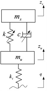
$m_s$ is the sprung mass of the car body, including passengers and internal components; it varies according to the number of passengers and the payload condition of the car. It is supported by the suspension system including air spring and damping adjustable absorber, and both of them have nonlinear characteristics. The shock absorber is a continuous adjustable damper. The damping force can be adjusted by controlling the current of solenoid valve according to a given logic. $m_u$ is the unsprung mass which is supported by the tire modeled as linear spring with stiffness coefficient $k_t$. The displacement of the sprung mass and unsprung mass are denoted as $z_s$ and $z_u$ respectively; and the road profile is denoted as $q$. So the dynamic equations of the nonlinear suspension can be described as:

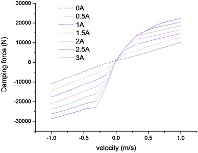
where, $F_s$ is the air spring force; which is the function of damper stroke, as shown in Fig. 2; $F_d$ is the damping force of the continuously adjustable damper; which is the function of damper stroke, stroke rate and the control current, as shown in Fig. 3. In the simulation, a 3-D look-up table model is created to describe the nonlinear characteristics of the adjustable damper.

Fig. 2The characteristic of the air spring force

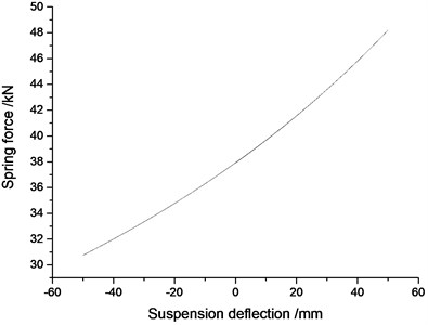
Fig. 3Damping force-velocity characteristics for different control currents

3. UKF observer design

Some suspension control algorithms assume that all states are measureable. But in practice, some states are either difficult to be measured or cannot be measured at all due to the high cost or limitations of technology. So it is necessary to design the observer to identify the states or parameters of the suspension systems. Many estimation algorithms for the nonlinear systems have been proposed in recent years, such as EKF [21], UKF [22], sliding mode observer [23] et al.

EKF is a nonlinear version of KF to optimally estimate the state information and parameters for the nonlinear systems. It is based on the Taylor series expansion theory and first order approximation to linearize the nonlinear system. This method induces a large error in the actual values of mean and covariance, which may lead to sub-optimal performance and sometimes even cause divergence of the filter [24]. Furthermore, it is difficult to calculate the Jacobi matrix during the system linearization especially for the strong nonlinear systems, such as the suspension with adjustable damper.

UKF is a nonlinear Kalman Filter which avoids calculating the Jacobi matrix and shows superior accuracy compared with the EKF which works with a linearized nonlinear model. It is based on the Unscented Transform (UT) theory and statistical linearization technique. This technique is a new approximation method by propagating means and covariance through nonlinear transformations. The UKF is better than the EKF in terms of robustness and speed of convergence; the computational load in applying the UKF is similar to the EKF [25].

3.1. UKF approach

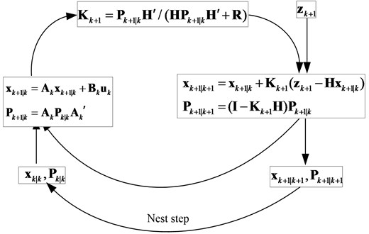
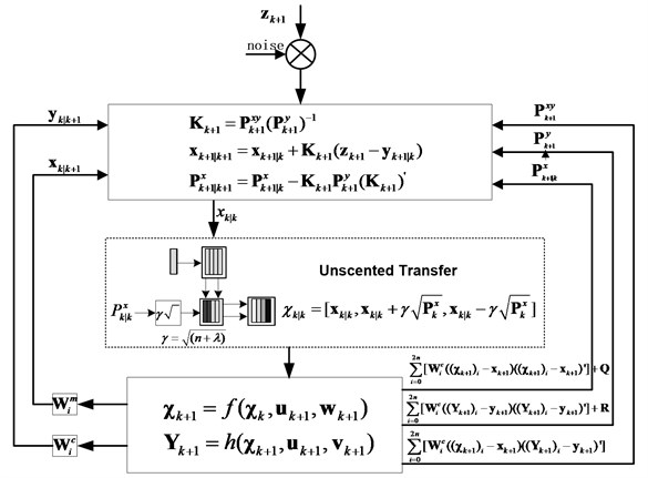
Fig. 4 is the flowchart of linear KF; and Fig. 5 is the flowchart of UKF theory. The unscented transfer is a mathematical tool for calculating the statistics of a random variable which undergoes a nonlinear transformation. The procedures of the algorithm can be organized as follows [18].

3.1.1. Sigma points calculation

The sigma points are a set of points which have mean and covariance equal to the given mean and covariance. The elements of sigma points are discrete in probability distribution. This distribution can be propagated exactly by applying the nonlinear function to each point.

In the paper, we use the symmetrically sampling method to pick up the sigma points. For the random variable state vector $\mathbf{x}$, the mean is $\stackrel{-}{\mathbf{x}}$ and the covariance of $\mathbf{x}$ is denoted as ${\mathbf{P}}^{\mathbf{x}}$. The sigma points are chosen so that their mean and covariance are exactly equal to $\stackrel{-}{\mathbf{x}}$ and ${\mathbf{P}}^{\mathbf{x}}$ respectively. Define ${\chi }_k$ as a set of $2N+1$ sigma points [26]:

5

${\chi }_k=\left\{\begin{array}{ll}\stackrel{-}{\mathbf{x}},& k=0,\\ \stackrel{-}{\mathbf{x}}+(\sqrt{\left(N+\lambda \right){\mathbf{P}}^{\mathbf{x}}}{)}_k,& k=\mathrm{1,2},\dots ,N,\\ \stackrel{-}{\mathbf{x}}-(\sqrt{\left(N+\lambda \right){\mathbf{P}}^{\mathbf{x}}}{)}_{k-N},& k=N+1,\dots ,\mathrm{}2N,\end{array}\right.$

where, $N$ is the dimension of the state vector $\mathbf{x}$; $\lambda ={\alpha }^2\left(N+\kappa \right)-N$ is a scaling parameter, the constant $\alpha$ determines the spread of the sigma around $\stackrel{-}{\mathbf{x}}$, and is usually set to a small value (1$\le \alpha \le$10^-4)); $\kappa \ge 0\text{,}$ it can make sure that the covariance matrix is positive definite. ${\left(\sqrt{\left(N+\lambda \right){\mathbf{P}}^{\mathbf{x}}}\right)}_k$ is the $i$th column of the matrix square root.

Fig. 4Flowchart of KF

3.1.2. Nonlinear system function

These sigma vectors are propagated through the nonlinear system function:

6

${\chi }_{k+1}={\chi }_k+f\left({\chi }_k,{\mathbf{u}}_{k+1},{\mathbf{w}}_{k+1}\right)\mathrm{\Delta }T,$

where, $\mathrm{\Delta }T$ is the sampling time; $f$ is the nonlinear system function; $u_{k+1}$ is the system control input; ${\mathbf{w}}_{k+1}$ is the process noise.

3.1.3. Measurements update

7

${\mathbf{Y}}_{k+1}=h\left({\mathbf{x}}_{k+1},{\mathbf{u}}_{k+1},{\mathbf{v}}_{k+1}\right),$

where, $h$ is measurement function; ${\mathbf{w}}_{k+1}$ is the measurement noise.

The mean of the state vector ${\mathbf{x}}_{k+1}$ and the measurement value ${\mathbf{y}}_{k+1}$ can be approximated by using a weighted sample mean of the sigma vectors:

8

${\mathbf{x}}_{k+1|k}\approx \sum _{i=0}^{2N}\left({\mathbf{W}}_{{\mathrm{}}_i}^m\right({\chi }_{k+1}{)}_i),{\mathbf{y}}_{k+1}\approx \sum _{i=0}^{2N}\left({\mathbf{W}}_{{\mathrm{}}_i}^m\right(Y_{k+1}{)}_i).$

Fig. 5Flowchart of UKF

3.1.4. Covariance update

The covariance of the state vector and the measurement vector can be updated by:

9

${\mathbf{P}}_{{\mathrm{}}^{{\mathrm{}}_{k+1|k}}}^{\mathbf{x}}=\sum _{i=0}^{2N}\left[{\mathbf{W}}_i^c\right(\left({\chi }_{k+1}{)}_i-{\mathbf{x}}_{k+1}\right)\left({\left({\chi }_{k+1}{)}_i-{\mathbf{x}}_{k+1}\right)}^{\mathrm{\text{'}}}\right]+\mathbf{Q},$
${\mathbf{P}}_{{\mathrm{}}^{{\mathrm{}}_{k+1}}}^{\mathbf{y}}=\sum _{i=0}^{2N}\left[{\mathbf{W}}_i^c\right(\left(Y_{k+1}{)}_i-{\mathbf{y}}_{k+1}\right)\left({\left({\mathbf{Y}}_{k+1}{)}_i-{\mathbf{y}}_{k+1}\right)}^{\mathrm{\text{'}}}\right]+\mathbf{R},$
${\mathbf{P}}_{{\mathrm{}}^{{\mathrm{}}_{k+1}}}^{\mathbf{x}\mathbf{y}}=\sum _{i=0}^{2N}\left[{\mathbf{W}}_i^c\right(\left({\chi }_{k+1}{)}_i-{\mathbf{x}}_{k+1}\right)\left({\left({\mathbf{Y}}_{k+1}{)}_i-{\mathbf{y}}_{k+1}\right)}^{\mathrm{\text{'}}}\right].$

The weight can be updated by:

10

${\mathbf{W}}_i^m=\left[\frac{\lambda }{N+\lambda },\underset{2N}{\underbrace{\frac{\frac{1}{2}}{N+\lambda },\cdots ,\frac{\frac{1}{2}}{N+\lambda }}}\right],\mathrm{}\mathrm{}$

11

${\mathbf{W}}_i^c=\left[\frac{\lambda }{N+\lambda }+1-{\alpha }^2+\beta ,\underset{2N}{\underbrace{\frac{\frac{1}{2}}{N+\lambda },\cdots ,\frac{\frac{1}{2}}{N+\lambda }}}\right],$

where, assuming that the system process noise and the measurement noise are Gaussian white noises, and the covariance of them are $\mathbf{Q}$ and $\mathbf{R}$ respectively. $\beta$ considers the high order moment of the prior distribution, for Gaussian distribution, $\beta =\mathrm{}$2 is optimal.

3.1.5. Correction

12

${\mathbf{K}}_{k+1}={\mathbf{P}}_{k+1}^{xy}{\left({\mathbf{P}}_{k+1}^y\right)}^{-1},{\mathbf{x}}_{k+1|k+1}={\mathbf{x}}_{k+1|k}+{\mathbf{K}}_{k+1}\left({\mathbf{z}}_{k+1}-{\mathbf{y}}_{k+1}\right),$
${\mathbf{P}}_{k+1|k+1}^x={\mathbf{P}}_{k+1|k}^x-{\mathbf{K}}_{k+1}{\mathbf{P}}_{k+1}^y({\mathbf{K}}_{k+1}{)}^{\mathrm{\text{'}}},$

where, ${\mathbf{z}}_{k+1}$ is the measurement signal from the sensors.

3.2. Suspension state estimation

Define the state vector as $\mathbf{x}=[{\dot{z}}_s,{\dot{z}}_u,z_s-z_u,z_u-q,z_s,z_u{]}^T$, and choose suspension stroke rate and stroke as observer measurements, i.e. $h\left(\mathbf{x}\right)=[{\dot{z}}_s-{\dot{z}}_u,z_s-z_u{]}^T$. The system dynamics can be rewritten in the format of state-space as:

13

$\left\{\begin{array}{l}\dot{\mathbf{x}}=f\left(\mathbf{x}\right)+\mathbf{G}\mathbf{w},\\ \mathbf{y}=h\left(\mathbf{x}\right)+\mathbf{v},\end{array}\right.$

where:

$f\left(\mathbf{x}\right)={\left[\begin{array}{llllll}-\frac{F_d}{m_s}-\frac{F_s}{m_s},& \frac{F_d}{m_u}+\frac{F_s}{m_u}-\frac{k_t}{m_u}{x}_4,& x_1-x_2,& x_2,& x_1,& x_2\end{array}\right]}^{{\rm T}},$
$\mathbf{G}=[\begin{array}{llllll}0& 0& 0& -1& 0& 0\end{array}{]}^{{\rm T}},$

represent the nonlinear system function and road disturbance matrix, respectively; $h\left(\mathbf{x}\right)={\left[\begin{array}{ll}{x}_1-x_2,& x_3\end{array}\right]}^{{\rm T}}$ represents the measurement outputs. $\mathbf{w}=\dot{q}$ is the process noise, which is the derivative of road disturbance and it is a white noise with covariance $\mathbf{Q}$; $v$ is the measurement noise assumed to be zero mean Gaussian white noise with covariance $\mathbf{R}$.

Where, $x_1={\dot{z}}_s$ – vertical velocity of sprung mass; $x_2={\dot{z}}_u$ – vertical velocity of unsprung mass; $x_3=z_s-z_u$ – relative displacement of suspension; $x_4=z_u-q$ – tire deflection; $x_5=z_s$ – vertical displacement of sprung mass; $x_6=z_u$ – vertical displacement of unsprung mass.

And the continuous-time nonlinear system Eq. (13) can be written as discrete-time nonlinear system function by using the first-order approximation, as shown in Eq. (14):

14

$\left\{\begin{array}{l}{\mathbf{x}}_{k+1}={\mathbf{x}}_{k+1}+\left(f\left({\mathbf{x}}_k\right)+\mathbf{G}{\mathbf{w}}_k\right)\mathrm{\Delta }T,\\ {\mathbf{y}}_{k+1}=h\left({\mathbf{x}}_{k+1}\right)+{\mathbf{v}}_{k+1}.\end{array}\right.$

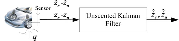
Based on the above system function and the UKF estimation theory, the state observer of nonlinear suspension system is designed, as shown in Fig. 6. Here the road disturbance is considered as system process noise. So the designed observer is of low sensitivity to unknown random road disturbances.

Fig. 6The flowchart of suspension state observer

3.3. Sprung mass identification

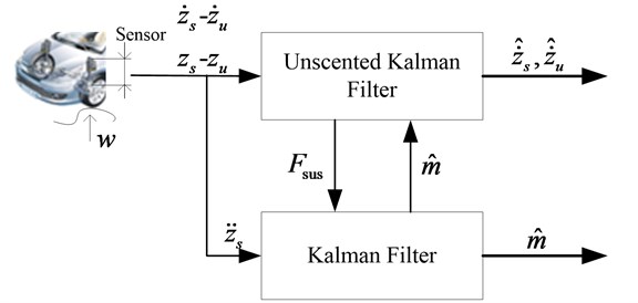
The sprung mass often changes with the number of the passengers, loaded or unloaded conditions. Thus the resonant frequency of the vibration system will change [27], and the ride comfort will reduce greatly if the corresponding adjustment of the suspension cannot be made. So it is meaningful to identify the sprung mass in real-time. The sprung mass estimator is designed based on the linear KF. And combined with the state observer which designed in Section 3.2; the two estimators exchange the estimated results simultaneously, as shown in Fig. 7. Assuming that the sprung mass is constant when vehicle is driving, we choose $\theta =1/\widehat{m}$ as the system state and the sprung mass acceleration as measurement. The estimation function can be described as:

15

$\left\{\begin{array}{l}{\theta }_{k+1}={\theta }_k+{\mathbf{w}}_{1k},\\ {\mathbf{y}}_{k+1}=\mathbf{H}{\mathrm{\theta }}_{k+1}+{\mathbf{v}}_{1k},\\ {\mathbf{w}}_1\stackrel{\mathrm{c}\mathrm{o}\mathrm{v}\mathrm{a}\mathrm{r}\mathrm{i}\mathrm{a}\mathrm{n}\mathrm{c}\mathrm{e}}{\to }{\mathbf{Q}}_1,\\ {\mathbf{v}}_1\stackrel{\mathrm{c}\mathrm{o}\mathrm{v}\mathrm{a}\mathrm{r}\mathrm{i}\mathrm{a}\mathrm{n}\mathrm{c}\mathrm{e}}{\to }{\mathbf{R}}_1,\end{array}\right.$

where, $\mathbf{H}$ is the suspension force from UKF estimator; $\mathbf{y}={\ddot{z}}_s$, is the measurement; ${\mathbf{w}}_{1k}$, ${\mathbf{v}}_{1k}$ are the process noise and the measurement noise in the sprung mass identification system, respectively.

Fig. 7The flowchart of suspension observer

4. Simulation and analysis

The efficiency of designed observer is verified through numerical simulations on two different typical road profiles, the random road and speed bump road, respectively. The random road represents consistent excitations with a wide range of frequencies; and the speed bump road represents the discrete events of relatively short duration and high intensity. The simulation parameters of the quarter car are listed in Table 1.

4.1. Case 1 random road excitation

In this section, the estimation efficiency is validated on random road excitation. The ISO has proposed a series of standards of road roughness classification by using the power spectral density (PSD) values (ISO 1982). The PSD of the random road excitation can be expressed as the following form:

16

$G_q\left(n\right)=G_q\left(n_0\right){\left(\frac{n}{n_0}\right)}^{-w},$

where, $n$ is the space frequency in m^-1; $n_0$ is the reference space frequency, $n_0=\mathrm{}$0.01 m^-1; $G_q\left(n_0\right)$ is the road roughness coefficient, here, $G_q\left(n_0\right)=\mathrm{}$256×10^-6; $w$ is frequency index, which reflects the frequency structure of the pavement, usually $w=\mathrm{}$2.

The model of road random excitation is built through integrated Gaussian white noise [28]. The equation of the random road in time domain can be expressed as:

17

$\dot{q}\left(t\right)=2\pi n_0\sqrt{G_q\left(n_0\right)u}W\left(t\right)-2\pi n_{00}uq\left(t\right),$

where, $W\left(t\right)$ is the Gauss white noise; $n_{00}$ is the low cut-off space frequency, $n_{00}=\mathrm{}$0.001 m^-1; $u$ is the vehicle speed.

The irregular road profile is shown in Fig. 8. The vehicle speed is kept constant as 20 m/s. The estimation results are shown in Fig. 9-Fig. 11.

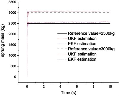
Fig. 9 and Fig. 10 are the comparison of UKF and EKF estimation results when vehicle is driving on the random road excitation. It is clearly indicated that the estimation results of UKF observer are more precise than those of EKF. Even though both of them have a short time delay, which is acceptable in engineering applications. Fig. 11 plots the results comparison of the sprung mass estimation when the vehicle is in unloaded and full load conditions, respectively. It can be found that both estimation methods work well.

Fig. 8The random road profile

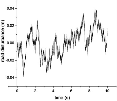
Fig. 9Comparison of the sprung mass velocity estimation results

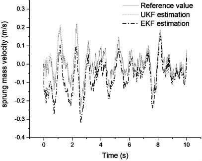
Fig. 10Comparison of the unsprung mass velocity estimation results

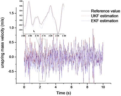
Fig. 11Comparison of the sprung mass estimation results

4.2. Case 2 speed bump road excitation

The speed bump road profile is shown in Fig. 12. The vehicle speed is kept constant as 5 m/s. The simulation results are shown in Figs. 13-14.

Fig. 13 and Fig. 14 are the comparison of suspension state estimation results when the vehicle is driving over a speed bump road. From Fig. 13, we can find that estimation result of sprung mass velocity from UKF observer is more precise compared with that from the EKF method.

Fig. 12The speed bump

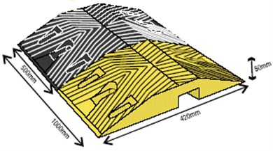
Fig. 13Comparison of the sprung mass velocity results

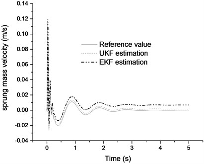
Fig. 14Comparison of the unsprung mass velocity results

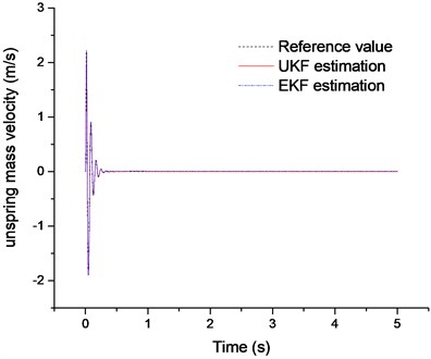
Fig. 15Errors analysis of estimation results

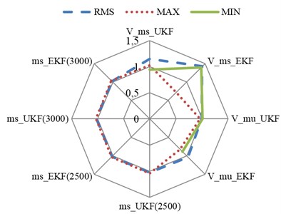
a) Random road condition

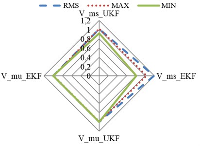
b) Speed bump road condition

5. Conclusions

An observer with low sensitivity to road disturbance is designed based on UKF theory for nonlinear suspension systems. The UKF observer is successfully in estimating the state information of the suspension vibration with good accuracy. The efficiency of the proposed estimator is validated on two typical road excitations and in the condition of sprung mass variation. Compared with the EKF observer, the simulation results indicated that the performance of the designed UKF observer is more precise, and the sprung mass estimator is also proposed combined with the designed suspension state estimator. The performance of the sprung mass estimator is validated on random road excitations and the estimation results are very satisfying. The future work will be concentrating on developing the states observer for full vehicle suspension considering pitch and roll motion and validating the designed observer algorithms in real vehicle tests.

6. Acknowledgements

The present work is supported by the National Nature Science Foundation of China (Grant Nos. 51375046, 51205021).