The contact mode of a joint interface based on improved deep neural networks and its application in vibration analysis

Tian, Yang; Liu, Zhifeng; Cai, Ligang; Pan, Guangyuan

doi:10.21595/jve.2016.16373

Journal of Vibroengineering

Browse Journal

Submit article

Published: 15 May 2016

Check for updates

The contact mode of a joint interface based on improved deep neural networks and its application in vibration analysis

Yang Tian¹

Zhifeng Liu²

Ligang Cai³

Guangyuan Pan⁴

¹Department of Research, Liaoning Engineering Vocational College, Liaoning Tieling 112000, China

^{1, 2, 3}Beijing Key Laboratory of Advanced Manufacturing Technology, Beijing University of Technology, Beijing 100124, China

⁴College of Electronic and Control Engineering, Beijing University of Technology, Beijing 100124, China

Corresponding Author:

Zhifeng Liu

Cite the article Download PDF

Downloads 1656

WoS Core Citations 3

CrossRef Citations 3

Abstract

The precision of the contact model for a joint interface strongly depends on the fractal dimension and fractal roughness coefficient. In this paper, an improved deep neural network method was adopted to predict the surface appearance parameters. In order to meet the high accuracy requirements for the prediction results of the contact model, a novel surface appearance prediction model was established utilizing a regularized deep belief network. The Bayesian regularization strategy was used to reduce the network weights during unsupervised training, which can effectively restrain the contribution of unimportant neurons. This allows to limit the occurrence of overfitting, and the layer-by-layer training was performed for each hidden layer based on a continuous transfer function. Meanwhile, the surface appearance parameters of the joint interface could be obtained by plugging arbitrary machining parameters into the training model. The specific contact model was then established based on fractal theory by applying the above-mentioned prediction results. The parameters of the joint interface were used to simulate the frequencies and vibration modes of frame-shaped structural parts. The contact model was validated by comparing the simulation results with experimental data. The proposed model is expected to provide a theoretical basis for optimizing the structure and improving the accuracy of computerized numerical control machines.

1. Introduction

High-strength bolting is the main type of fixed connection for the structural parts of computerized numerical control (CNC) machines. The dynamic and static characteristics of their joint parts are the key factors influencing the accuracy and reliability of heavy CNC machine tools. Studies on the influence of the joint part on the overall performance of the machine tool have shown that it reduces the integral rigidity and increases the damping [1]. About 30 to 50 % of the rigidity of the machine tool depends on the stiffness of the joint part, while more than 90 % of the damping of the machine tool is also due to the joint part.

The joint interface consists of two rough surfaces in contact with each other. At present, in theoretical models, the joint interface is commonly simplified to a contact problem between an equivalent rough surface and a rigid plane [2, 3]. Therefore, calculating the fractal parameters for the equivalent rough surface is essential for obtaining the contact stiffness of the joint interface. A variety of studies have been conducted to establish suitable contact models. For instance, based on statistical analysis, Greenwood and Williamson established the so-called G-W contact model for rough surfaces [4], which considers the appearance parameters of the rough surface. They found that the distribution of the surface height values of many rough surfaces can be described by a Gauss distribution and that a rough surface can be described as consisting of many micro-bulges with the same curve radius but different heights.

Majumdar and Bhushan proposed the so-called MB contact model based on fractal geometry [5]. The fractal dimension $D$ and the fractal roughness coefficient $G$ were adopted in the MB model to represent the rough surface. The distribution function in the MB model describes the distribution of the size of the flat cross-sectional area in a single micro-bulge in case the two rough surfaces were in contact with each other. Zhang et al. [6] established an elastic-plastic fractal model to calculate the energy dissipation occurring in case of tangential contact damping at a joint interface as a function of the stretch factor in the distributed domains of the micro-contact area, and analyzed how the fractal dimension D influences the damping loss.

Based on the three-dimensional fractal characterization method and the assumption that the cross-sectional contact area of the micro-bulges followed an exponential distribution, Komvopoulos established a rigid sphere and a semi-infinite finite element contact model for an elastic-plastic isotropic medium [7], which was used to determine the relationship between the actual contact area and the corresponding deformation under the average contact pressure and was successfully applied to model a multilayered medium. Tian et al. [8] reported on a method to identify the fractal dimension and fractal roughness of a joint part, and corrected the formula for calculating the normal gross load on the joint part. Jiang et al. [9] calculated the fractal parameters of a rough surface by utilizing the structure function on the basis of three dimensional fractal contact theory. Considering the distribution function of the micro-bulge’s cross-sectional area, the total normal and tangential contact rigidities of the joint interface were computed by calculating the normal and tangential contact rigidity of a single micro-bulge. Furthermore, they compared the theoretical total normal and tangential contact rigidities of a joint interface with experimental results.

Yan expanded the two-dimensional characterization of a rough surface to a three-dimensional characterization method, combining it with the elastic-plastic contact mechanism [10]. He derived the relationship between the total normal force and the actual contact area, as well as the relationships between the three-dimensional characterization and the fractal parameters, the material characteristics and the average distance between the surfaces. Wen et al. proposed a calculation method on the assumption that the interface parameters of the joint part are equivalent to the fractal parameters of the profile of the rough surface, and established a model for the tangential contact rigidity of a joint part. By studying the contacting process between two rough surfaces, Liou [12] observed that the fractal dimension $D$ and the fractal roughness parameter $G$ are related to the relative distance d between the two surfaces. Wang further corrected the distribution function for the contact area of the micro-bulges in the MB model [13], and performed a three-dimensional appearance analysis on the profile of the rough surface. An accurate model of the surface appearance of a joint interface is the most important premise for studying the contact parameters of a joint interface. However, applying traditional statistical analysis methods results in a low accuracy of the predicted appearance of the machined surface. Therefore, in this paper, a regularized deep belief network (rDBN) surface appearance prediction model was first established based on the deep neural network (DNN) method, and arbitrary data collected by a high-precision topography instrument was then plugged into the model to determine the surface appearance parameters of the joint interface. The precision of the prediction model was verified by comparison with the test samples. Then, by adopting fractal theory and the Hertz contact theory, the finite element method (FEM) was employed to establish a model for the contact rigidity, and a damping model of the joint interface was derived. These models were then applied to the simulation software. Finally, the contact model was validated by comparing the theoretical data with the frequencies and vibration modes of frame-shaped structural parts determined through modal testing experiments under different pretension forces.

2. Regularized deep belief network model

The relationship between processing parameters and surface morphology parameters is usually difficult to express as a mathematical formula. Ordinary models also fail to establish such a relationship; however, DBN presents good non-linear mapping capabilities and its internal computing mechanism can serve as a black-box model which is not taken into account. By adjusting the weights of DBN during training, the non-linear mapping of input and output variables can be realised so as to indirectly acquire the surface morphology parameters (output variables) through known processing parameters (input variables).

According to fractal theory, a rough surface can be described by the fractal dimension $D$ and the fractal roughness coefficient $G$ . Thus, a prediction model must be established consisting of the machining parameters as the input layer and the fractal dimension $D$ and the fractal roughness coefficient $G$ as the output layer. By plugging the machining parameters of the joint interface into the model, a prediction of fractal parameters can then be obtained. The contact parameters of the joint interface strongly depend on the accuracy of the fractal parameters. To achieve a high accuracy, a prediction model based on a regularized deep belief network (rDBN) is proposed in this paper.

2.1. Structure of the neural network

A rDBN consisting of several super-imposed Restricted Boltzmann Machines (RBMs) is proposed with an added regularization item and an output layer (Fig. 1) to compare the labels. The RBMs feature a visible layer V and a hidden layer H, as shown in Fig. 1.

Fig. 1Schematic illustration of the structure of the proposed rDBN

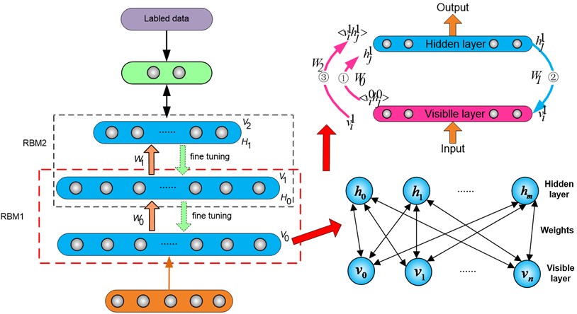
The visible layer provides for the input part during the training process, in which we use a Simulated Annealing (SA) algorithm, while the output part (the layer that follows the hidden layer) is used for data comparison; its weights were determined through back propagation. The structure of the network consists of full two-way connections between $V$ and $H$ , whereas no connections exist between units of the same layer. The absence of intra-layer connections results in a “restricted” Boltzmann Machine. During the training process, each hidden layer extracts the previous layer’s data information and features in order to form a better but more abstract distributed representation of the input data. The last layer provides the output, and contains several units of classification.

The training process of the rDBN can be described as follows: Firstly, each RBM is individually trained unsupervised. The input of each RBM is the output of the previous layer. Contrastive Divergence (CD) was applied to train one hidden layer at a time, while, at the same time, an improved Bayesian regularization item, i.e., the regularization term, was added to the reasoning and generation processes. This special regularization term can help to reduce overfitting and comprises the sum of the squares of the weights. It ensures that the optimization process not only achieves the objective of the minimization of the error metric, but also that the objective is achieved with minimum-magnitude weights. Next, supervised training is then used to fine-tune the whole network after the BP in the last layer received a signal from the last RBM. The regularization term can be omitted in this training step because the unsupervised training already ensures that the initial area is good enough, and the iterations of the supervised training can then be evaluated empirically.

2.2. The neural network algorithm

In a rDBN, several RBMs are stacked layer by layer, and each RBM is trained individually during the unsupervised training using Markov Chain Monte Carlo (MCMC) and CD methods, and a new objective function responsible for weight-control and regularization will be introduced. Since there are no connections between hidden units in an rDBN, the behavior of the hidden units as a function of the behavior of the visible units can be expressed as:

1

p (h_{j} = 1) = \frac{1}{1 + e x p (- b_{j} - \sum_{i} v_{i} w_{i j})} .

Because the RBM in an rDBN is symmetrical and since there are no visible-visible connections, the behavior of the visible units as a function of the hidden units can be similarly expressed as:

2

p (v_{i} = 1) = \frac{1}{1 + e x p (- c_{i} - \sum_{j} h_{j} w_{j i})},

where $v_{i}$ is the value of unit $i$ in the visible layer, $h_{j}$ is the value of unit $j$ in the hidden layer, $b$ and $c$ are the biases of $V$ and $H$ , respectively, $w_{j i}$ is the weight between the visible unit $i$ and the hidden unit $j$ , and $p ()$ denotes the probability that the identified unit is in state “1”.

In a binary RBM, the weights on the connections and the biases of the individual units define a probability distribution over the joint states of the visible and hidden units which can be written as an energy function: $E (v, h) = h^{T} W v + b^{T} v + c^{T} h$ . The joint probability distribution of the characteristic vector $v$ in the visible layer $V$ and $h$ in the hidden layer $H$ can be expressed as:

3

P (v, h) \propto e x p (- E (v, h)) = e^{h^{T} W v + b^{T} v + c^{T} h},

where $W$ is the weight matrix between $V$ and $H$ , and $E (v, h)$ is the joint expectation of $v$ and $h$ ; its absolute value corresponds to the amount of information $h$ receives from $α$ . The ideal parameters $θ = (W, b, c)$ that result in a peak joint probability distribution $p (v, h)$ [14] can be calculated through the maximum likelihood method. However, this method often fails to yield the exact value of $θ .$ Therefore, an MCMC method that renews $V$ and $H$ individually is often employed. The parameter vector $θ$ is gradually modified along the gradient of $p (v, h)$ according to the following equation:

4

θ^{(τ + 1)} = θ^{(τ)} + η \frac{\partial l o g P (v, h)}{\partial θ},

where $τ$ is the iteration number, which depends on the network size (as large as $τ =$ 100-2000), and $η$ is the learning speed that affects the speed of convergence. Choosing an appropriate value of $η$ can affect both the speed of convergence and the accuracy of the solution.

Let $v_{i}^{m}$ be the state vector of the visible unit $i$ at time $t = m$ . For example, $v^{0}$ is the state vector at $t = 0$ (the input of the RBM), and $h^{0}$ is the state vector of the hidden layer that is a function of $v^{0}$ and obtained through Eq. (1). Then, $v^{1}$ is the state vector at $t = 1$ depending on $h^{0}$ and obtained through Eq. (2), and so on. $v^{\infty}$ and $h^{\infty}$ are the state vectors at $t = \infty$ (steady state). The slope in Eq. (4) can be calculated as follows:

5

\frac{\partial l o g P (v, h)}{\partial θ_{i j}} = 〈h_{j}^{0} (v_{i}^{0} - v_{i}^{1})〉 + 〈v_{i}^{1} (h_{j}^{0} - h_{j}^{1})〉 + \dots = 〈h_{j}^{0} v_{i}^{0}〉 - 〈h_{j}^{\infty} v_{i}^{\infty}〉,

where $〈h^{0} v^{0}〉$ is the dot product average of $v^{0}$ and $h^{0}$ , and $〈h^{\infty} v^{\infty}〉$ , which is convergent, is the value at the end point of the MCMC. When applying the CD method [15], $〈h_{j}^{0} v_{i}^{0}〉$ is the joint probability distribution of the data, and $〈h_{j}^{\infty} v_{i}^{\infty}〉$ is in fact $〈h_{j}^{1} v_{i}^{1}〉$ , which means a reconstruction of the input data, because only one Gibbs sampling algorithm is used for the two layers. According to Eq. (5), the slope only depends on the initial state and the final state. Thus the formula to renew the weights can be expressed as:

6

θ^{(τ + 1)} = θ^{(τ)} + η \frac{\partial l o g P (v, h)}{\partial θ} = θ^{(τ)} + η (〈h_{j}^{0} v_{i}^{0}〉 - 〈h_{j}^{1} v_{i}^{1}〉) .

Training a network using only a limited amount of samples is an ill-posed problem. There are many potential models that can meet the set performance (i.e., resulting in a response very close to the expected response). In order to choose one of the possible alternatives, the problem needs to be regularized by selecting additional conditions apart from the requirement that the response of the trained network must be in agreement with the expected response. In Bayesian regularization [16], the imposed additional objective ensures that the selected trained network not only minimizes the error metric but also achieves this objective with minimum-magnitude weights. In a rDBN, since the values the hidden units can attain are discrete, i.e., either 0 and 1 during training, the regular form of Bayesian cannot be directly applied, and therefore the objective function presented in Eq. (3) above was modified as follows:

7

F_{W} = α P + β E_{W},

where $F_{W}$ is the new objective function during unsupervised training, and $P$ is the original objective function given in Eq. (3). In Eq. (7), $E_{W}$ is the regularization item, $α$ and $β$ are performance parameters that need to be calculated during the iterations or must be set prior to the iteration. $E_{W}$ has the form of the mean square of the weights. $P$ and $E_{W}$ can be expressed as:

8

P = P (v, h) \propto e x p (- E (v, h)) = e^{h^{T} W v + b^{T} v + c^{T} h},

9

E_{W} = \frac{1}{m \times n} \overset{m}{\sum_{j = 1}} \overset{n}{\sum_{i = 1}} w_{i j}^{2},

where $w_{i j}$ denotes the weight between $i$ in the visible layer and $j$ in the hidden layer. If $α ≫ β$ , the first part of $F_{W}$ dominates, which means that the objective of the training is to decrease the training error. Specifically, if $α = 1$ , $β = 0$ , then $F_{W} = P$ . On the other hand, if $α ≪ β$ , the training will focus on decreasing the weights. By introducing this regularization item, the weights not contributing to the response will be minimized, which ensures that only those parts of the network learning the “important” features that are common to all the input patterns will remain. Therefore, an improvement in the response of the trained network is expected for arbitrary test inputs.

The traditional way of training Bayesian regularization is based on the calculation of $α$ and $β$ during the training process [17]. The weights are treated as random variables, and the prior probabilities of $P$ and $E_{W}$ are assumed to follow a Gaussian distribution. Then, $α$ and $β$ can be obtained using the Bayes criterion. The hidden neurons in an RBM only attain discrete values (0 and 1), and therefore the Hessian matrix cannot be calculated. The appropriate values of $α$ and $β$ must be determined experimentally. For this modified unsupervised training process, Eq. (7) must be transformed to:

10

F_{w}^{'} = \frac{\partial l o g P (v, h)}{\partial θ} + \frac{2}{m \times n} \overset{m}{\sum_{j = 1}} \overset{n}{\sum_{i = 1}} w_{i j},

and the behavior of the reasoning and output generation equations is given by:

11

F (h_{j} = 1) = \frac{1}{1 + e x p (- b_{j} - \sum_{i} v_{i} w_{i j})},

12

F (v_{i} = 1) = \frac{1}{1 + e x p (- c_{i} - \sum_{j} h_{j} w_{j i})} .

In order to realize a prediction model for continuous numerical values, in this study, the unsupervised training transfer function of the rDBN and the transfer function were improved for the unsupervised training process. Furthermore, a continuous unsupervised operation approach is proposed. Here, $s_{j}$ and $s_{i}$ denote the neuron $j$ of the hidden layer and the neuron $i$ of the visible layer, respectively. Whereas the transfer functions of the sigmoid in Eqs. (1) and (2) are maintained, the discretization process is removed. Furthermore, a noise variable was added to realize the transformation to continuous numerical values. This yields:

13

s_{j} = φ_{j} (\sum_{i} w_{i j} s_{i} + σ N_{j} (0,1)),

14

s_{i} = φ_{i} (\sum_{i} w_{i j} s_{j} + σ N_{i} (0,1)),

and:

15

φ_{j} (x_{j}) = θ_{L} + (θ_{H} - θ_{L}) \frac{1}{1 + e^{- a_{j} x_{j}}},

16

φ_{i} (x_{i}) = θ_{L} + (θ_{H} - θ_{L}) \frac{1}{1 + e^{- a_{i} x_{i}}} .

Eq. (13) and (14) describe the learning and reasoning processes of the rDBN, respectively. Here, $N (0,1)$ denotes the Gaussian random variable with an average value of 0 and a variance of 1. $σ$ is a constant, and $φ ()$ is the sigmoid function with the asymptotic lines of $θ_{H}$ and $θ_{L}$ . $a$ is the noise control variable, which controls the slope of the sigmoid function. According to the CD criterion, the update formula of the weights and the offset values can be written as:

17

Δ w_{i j} = η_{w} (〈s_{i}^{0} s_{j}^{0}〉 - 〈s_{i}^{1} s_{j}^{1}〉),

18

Δ b = \frac{η_{b}}{b^{2}} (〈{s_{j}^{0}}^{2}〉 - 〈{s_{j}^{1}}^{2}〉),

19

Δ c = \frac{η_{c}}{c^{2}} (〈{s_{i}^{0}}^{2}〉 - 〈{s_{i}^{1}}^{2}〉),

where $η_{w}$ , $η_{b}$ and $η_{c}$ are the learning rates, while the definition of $〈〉$ is as before.

It is easy to notice that changing the object function will not change the two calculation processes between the visible layer and the hidden layer, which means that the upper and lower bounds of the output will not be affected, because the two parameters in Eq. (7) only affect their proportion; they have no effect on the boundaries of the transfer functions. Therefore, the convergence of the rDBN is assured.

3. Application of the prediction model

3.1. Training samples

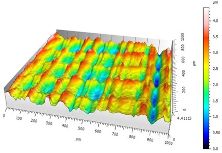
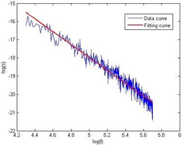
For the same network structure, an increase of the number of training samples can improve the prediction accuracy to some extent but also increases the test time. The total number of samples is typically in the range from 30 to 300 [18]. In literature, a 7:3 ratio of the number of training samples to the number of test samples is usually recommended. Therefore, the total sample capacity was selected to 77 in this study, with 54 training samples and 23 test samples. The training experiment consisted of two parts. In the first part (group 1-36), an integrated model experiment with five exercise factors at mixed levels was adopted for the milling process (with $v_{c}$ denoting the cutting speed, $f_{z}$ the feed per tooth, $a_{p}$ the axial cutting depth, $r_{e}$ the corner radius, and four factors). The feed and the rotating speed of the workpiece were arranged at three levels, respectively, and the axial cutting depth and the corner radius were arranged at two levels, respectively. For the other part of the training process (groups 37-54), an integrated model experiment with three exercise factors at mixed levels was applied to the grinding process (with $v_{c}$ denoting the rotating speed of the workpiece, $f_{z}$ the feed, and $a_{p}$ the axial cutting depth). The feed and the rotating speed of workpiece were arranged at three levels, respectively, whereas the axial cutting depth was arranged at two levels. Rectangular steel alloy blocks with dimensions of 30 mm×30 mm×40 mm were used as test specimens in this study, and the top surface was selected as the measuring surface. 77 groups of training and learning samples were obtained by adopting different milling processes. After machining, the workpieces were first cleaned under ultrasound in an alcoholic solution for 15 min. After cleaning, the workpieces were blow-dried with compressed air [19]. Then, a three-dimensional test instrument (Taylor CCI-lite) was used to measure and analyze the surface appearance, and the power spectral density of the surface data was obtained using Matlab. Finally, the fractal dimension $D$ and the fractal roughness coefficient $G$ were obtained for the different cutting processes. As shown in Fig. 2, the slope is determined by the fractal dimension $D,$ while the intercept is determined by the fractal roughness coefficient $G$ .

Fig. 2Calculation of the fractal parameters of the machined surfaces

$Calculation of the fractal parameters of the machined surfaces$

3.2. Experimental results

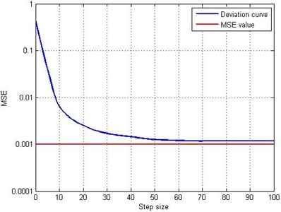
The purpose of the experiments was to test the function approximation ability of the rDBN and obtain a more accurate fractal dimension $D$ and fractal roughness coefficient $G$ by using an rDBN for the prediction of the surface appearance parameters. In the experiments, the network input was the real surface data in time sequence. In present theory, there is no unified method to determine the required number of hidden layer neurons for deep belief networks. Different issues require a different number of neurons, therefore the number of neurons is usually selected by experience during the experiment. Meanwhile, the network output is a neuron, which means the predicted data. For the experiments, the number of hidden layers was set to 2, and 20 neurons were included in every hidden layer. The number of unsupervised training iterations was selected to 50. After several trial runs, the regularization parameters were set to $α = 0.8$ , $β = 0.2$ , and the number of supervised training steps was set to 100. The required training accuracy was MSE = 0.001. Fig. 3 shows the training error curve obtained for the rDBN model.

Fig. 3The training error curve obtained for the rDBN model

The predicted values, the measured date and the relative errors of four test samples are shown in Table 1 for four test samples. It can be seen that the relative errors are controlled to be lower than 5 %; the maximum relative error between the measured and predicted values was 4.1 % and the minimum relative error was 0.47 %. This shows that the predicted surface appearance parameter values are comparatively accurate. A comparison of the results obtained for the test samples is shown in Fig. 1.

Table 1Comparison of the predicted and measured results for four test samples

		Experiment number
		1		2		37		38
		$D$	$G$	$D$	$G$	$D$	$G$	$D$	$G$
Surface appearance parameter	Measured value	2.3816	1.58e-12	2.3138	4.57e-12	2.4409	1.64e-11	2.3994	3.84e-11
Surface appearance parameter	Predicted value	2.4755	1.64e-12	2.2318	4.38e-12	2.4911	1.67e-11	2.4106	3.88e-11
Relative error %		2.5	3.7	–3.5	–4.1	2.05	1.8	0.47	1.04

4. Contact model

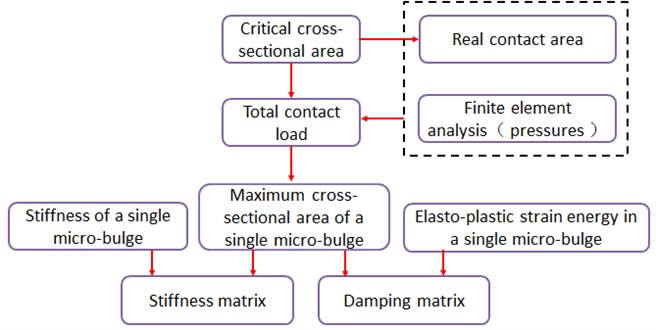
According to the predicted fractal dimensions and fractal roughness coefficient, fractal theory was used to simplify the joint interface contact into a stiffness and damping model by considering the influences of factors including the morphology of, the material properties of, and the external load on, the joint interface. To investigate the characteristics of the joint interface under non-uniform pressure, finite element analysis software was used to calculate the pressures on different elements in the joint interface, and the resulting pressures were taken as inputs to derive the stiffness and damping matrices. The process of deriving the stiffness and damping matrices is shown in Fig. 4 and can be described as:

1) Based on the formula for the distribution of the sizes of the critical cross-sectional area and the distribution of the cross-sectional area of the micro-bulges, the real contact area of the joint interface was deduced. Besides, the relationship between the total contact load and the maximum cross-sectional area of a single micro-bulge was also derived.

2) By acquiring the pressures on the different elements of the joint interface by static finite element analysis, the total contact load can be obtained by multiplying the pressures by the real contact area.

3) The total contact load found in Step 2, and the calculated relationship between the total contact load and the maximum cross-sectional area of a single micro-bulge found in Step 1, were combined to calculate the maximum cross-sectional area of single micro-bulge.

4) According to the stiffness of a single micro-bulge derived from on the definition of stiffness, the global stiffness matrix of the contact elements can be found by taking the maximum cross-sectional area of a single micro-bulge, and the critical contact area as the upper and lower limits of the integral.

5) By calculating the elasto-plastic strain energy in a single micro-bulge, the elasto-plastic strain energy of the contact element was found by taking the maximum cross-sectional area of a single micro-bulge, and the critical contact area as the upper and lower limits of the integral: the damping matrix was then deduced from the relationship between the damping and the stiffness.

Fig. 4process of deriving the stiffness and damping matrices

4.1. The real contact area model for the joint interface

According to the Hertz contact theory, the critical cross-sectional area, i.e., the area when the deformation mechanism of a micro-bulge changes from elastic deformation to plastic deformation, can be expressed as [20]:

20

a_{c}^{'} = {[\frac{2^{11 - 2 D} G^{2 (D - 2)} (l n γ) E^{* 2}}{π^{4 - D} (k H)^{2}}]}^{\frac{1}{D - 2}},

where $H$ is the hardness of the softer material. Here, $H = 2.8 Y$ , with $Y$ denoting the yield strength of the softer material. In Eq. (20), $E^{*}$ is the equivalent elastic modulus of the two different contacting materials, $k$ is the coefficient related to the Poisson’s ratio of the material, given by $k = 0.454 + 0.41 ν,$ where $ν$ is the Poisson’s ratio of the softer material. According to three-dimensional fractal theory, the distribution of the cross-sectional area of the micro-bulges is given by:

21

n (a^{'}) = \frac{D - 1}{2} {a_{l}^{'}}^{\frac{D - 1}{2}} a'^{\frac{- D - 1}{2}},

where $a'$ is the cross-sectional area of a micro-bulge, $a_{l}^{'}$ is the maximum of $a'$ .

According to Eq. (20) and Eq. (21), the total real contact area of the joint interface can be expressed as:

22

A_{r} = \{\begin{array}{l} \int_{0}^{a_{l}^{'}} a n (a^{'}) d a^{'} = \frac{D - 1}{2 (3 - D)} {a_{l}^{'}}^{\frac{D - 1}{2}} ({a_{l}^{'}}^{\frac{3 - D}{2}} + {a_{c}^{'}}^{\frac{3 - D}{2}}), a_{l}^{'} > a_{c}^{'}, \\ \int_{0}^{a_{c}^{'}} a n (a^{'}) d a^{'} = \frac{D - 1}{3 - D} {a_{l}^{'}}^{\frac{D - 1}{2}} {a_{c}^{'}}^{\frac{3 - D}{2}}, 0 < a_{l}^{'} < a_{c}^{'}, \end{array}

where $a$ is the critical real contact area of a single micro-bulge, and in fully elastic and plastic regime has different relationships with the cross-sectional area that can be expressed as $a = a' / 2$ , $a = a'$ , respectively.

For a fully elastic contact, the normal load of a micro-bulge can be given as $F_{e} = 4 / 3 E^{*} R^{1 / 2} δ^{3 / 2}$ . Then the total contact load perpendicular to the joint interface can be written as [21]:

23

P_{e} = \int_{a_{c}^{'}}^{a_{l}^{'}} F_{e} n (a') d a'

= \{\begin{array}{l} \frac{2^{\frac{(11 - 2 D)}{2}}}{3 π^{\frac{(4 - D)}{2}}} \cdot \frac{D - 1}{5 - 2 D} (l n γ)^{\frac{1}{2}} G^{(D - 2)} E^{*} {a_{l}^{'}}^{\frac{D - 1}{2}} ({a_{l}^{'}}^{\frac{5 - 2 D}{2}} - {a_{c}^{'}}^{\frac{5 - 2 D}{2}}), D \neq 2.5, \\ 2 π^{\frac{- 3}{4}} (l n γ)^{\frac{1}{2}} G^{\frac{1}{2}} E^{*} {a_{l}^{'}}^{\frac{3}{4}} l n (\frac{a_{l}'}{a_{c}'}), D = 2.5, \end{array}

and for a fully plastic contact, the normal load of a micro-bulge can be given as $F_{p} = H a'$ . Then the total contact load perpendicular to the joint interface is given by:

24

P_{p} = \int_{0}^{a_{c}^{'}} F_{p} n (a') d a' = \frac{H (D - 1) {a_{l}^{'}}^{\frac{D - 1}{2}}}{3 - D} {a_{c}^{'}}^{\frac{3 - D}{2}}

Thus, the total contact load perpendicular to the joint interface can be expressed as:

25

P = \{\begin{array}{l} P_{e} + P_{p}, a_{l}^{'} > a_{c}^{'}, \\ P_{p}, 0 < a_{l}^{'} < a_{c}^{'} . \end{array}

4.2. Normal contact rigidity model for the joint interface

The curvature radius and the normal deformation of a single micro-bulge can be expressed as [21]:

26

R = \frac{a'^{\frac{(D - 1)}{2}}}{2^{5 - D} π^{\frac{(D - 1)}{2}} G^{D - 2} {(l n γ)}^{\frac{1}{2}}},

27

δ = 2 G^{D - 2} {(l n γ)}^{\frac{1}{2}} {(2 r')}^{3 - D},

respectively, where $γ$ denotes the scale parameter. Considering the surface flatness and the spectral distribution density, $γ = 1.5$ . In Eq. (27), $r'$ is the radius of the cross-sectional area, which satisfies $r'^{2} = 2 R δ (R ≫ r')$ .

Therefore, when the micro-bulge is subject to a fully elastic contact, the normal contact rigidity of a single micro-bulge can be written as:

28

k_{n e} = \frac{d F_{e}}{d δ} = \frac{d F_{e}}{d a'} \frac{d a^{'}}{d δ} = \frac{4 E^{*} (4 - D)}{3 \sqrt{π} (3 - D)} a^{\frac{1}{2}} .

Integrating Eq. (28) then yields the total contact rigidity normal to the joint interface for a fully elastic contact:

29

K_{n e} = \int_{a_{c}^{'}}^{a_{l}^{'}} k_{n e} n (a^{'}) d a^{'} = \frac{2 \sqrt{2} E^{*} (4 - D) (D - 1)}{3 \sqrt{π} (3 - D) (2 - D)} {a_{l}^{'}}^{\frac{D - 1}{2}} ({a_{l}^{'}}^{\frac{2 - D}{2}} - {a_{c}^{'}}^{\frac{2 - D}{2}}) .

As a result, the total contact rigidity normal to the joint interface can be expressed as:

30

K_{n} = \{\begin{array}{l} K_{n e}, a_{l}^{'} > a_{c}^{'}, \\ 0, 0 < a_{l}^{'} < a_{c}^{'} . \end{array}

4.3. Tangential contact rigidity model for a joint interface

The tangential deformation at the joint interface for a micro-bulge can be expressed as [21]:

31

δ_{t} = \frac{3 μ p}{16 G^{*} r} [1 - {(1 - \frac{t}{μ p})}^{\frac{2}{3}}],

where $G^{*}$ is the equivalent shear modulus of the contacted material, $μ$ is the friction coefficient, $r$ is the radius of the real contact region, $p$ is the normal load acting on a single micro-bulge, and $t$ is the tangential load acting on a single micro-bulge. The ratio of the tangential load and normal load can be expressed as [22] $t / p = T / P$ , and $T$ is the total tangential load witch can be given as $T = τ_{b} A_{r}$ ( $τ_{b}$ is the shear strength).

Therefore, the tangential contact rigidity of a single micro-bulge is given by [23]:

32

t = μ p [1 - {(1 - \frac{16 G^{*} r δ_{t}}{3 μ p})}^{\frac{3}{2}}] .

Integrating Eq. (32) yields the total contact rigidity tangential to the joint interface for a fully elastic contact:

33

K_{t e} = \frac{4 \sqrt{2} G^{*} (D - 1)}{π^{\frac{1}{2}} (2 - D)} {(1 - \frac{T}{μ P})}^{\frac{1}{3}} {a_{l}^{'}}^{\frac{D - 1}{2}} ({a_{l}^{'}}^{\frac{2 - D}{2}} - {a_{c}^{'}}^{\frac{2 - D}{2}}) .

Thus, the total contact rigidity tangential to the joint interface can be expressed as:

34

K_{t} = \{\begin{array}{l} K_{t e}, a_{l}^{'} > a_{c}^{'}, \\ 0, 0 < a_{l}^{'} < a_{c}^{'} . \end{array}

4.4. Normal contact damping model for a joint interface

Assuming that $δ^{'}$ is the transient deformation of a single micro-bulge, the elastic strain energy can be expressed as:

35

ω_{e} = \int_{0}^{δ} F_{e} d δ' = \frac{2 \sqrt{2} E^{*} (3 - D)}{3 (7 - 2 D)} {(\frac{δ}{2^{4 - D} G^{D - 2} (l n γ)^{\frac{1}{2}}})}^{\frac{1}{(3 - D)}}

= \frac{2^{\frac{(19 - 4 D)}{2}} G^{2 (D - 2)} (l n γ) E^{*} (3 - D)}{3 π^{\frac{(7 - 2 D)}{2}} (7 - 2 D)} {a'}^{\frac{(7 - 2 D)}{2}} .

Therefore, the total elastic strain energy of the joint interface contact area can be written as follows:

36

W_{e} = \int_{a_{c}^{'}}^{a_{l}^{'}} ω_{e} n (a') d a'

= \frac{2^{\frac{(19 - 4 D)}{2}} E^{*} G^{2 (D - 2)} (l n γ) (3 - D) (D - 1)}{3 π^{(7 - 2 D)} (7 - 2 D) (8 - 3 D)} {a_{l}^{'}}^{\frac{(D - 1)}{2}} ({a_{l}^{'}}^{\frac{(8 - 3 D)}{2}} - {a_{c}^{'}}^{\frac{(8 - 3 D)}{2}}) .

Then, the plastic deformation energy of a single micro-bulge is given by:

37

ω_{p} = \int_{0}^{δ} F_{p} d δ^{'} = \frac{2^{(3 - D)} H G^{(D - 2)} (l n γ)^{1 / 2} (D - 1)}{(5 - D) π^{\frac{(3 - D)}{2}}} {a_{l}^{'}}^{\frac{(D - 1)}{2}} {a_{c}^{'}}^{(3 - D)} .

Thus, the total plastic strain energy of the joint interface contact are amounts to:

38

W_{p} = \int_{0}^{a_{c}^{'}} ω_{p} n (a') d a^{'} = \frac{2^{(2 - D)} H (1 - D) G^{(D - 2)} (l n γ)^{\frac{1}{2}}}{π^{\frac{(3 - D)}{2}} (5 - D)} {a_{l}^{'}}^{\frac{(D - 1)}{2}} {a_{c}^{'}}^{\frac{3 (3 - D)}{2}} .

Finally, the contact damping factor of the joint interface can be written as:

39

η_{n} = \{\begin{array}{l} \frac{W_{e}}{W_{p}}, a_{l}^{'} > a_{c}^{'}, \\ 0, 0 < a_{l}^{'} < a_{c}^{'} . \end{array}

Suppose that the mass of the entity containing the joint surface is $M$ . Then, the normal contact damping coefficient can be written as:

40

C_{n} = η_{n} \sqrt{M K_{n}} .

4.5. Tangential contact damping model for the joint interface

Assuming that $δ_{t}^{'}$ is the transient tangential deformation of the joint interface contact area, when the tangential force $t$ acts on a single micro-bulge for one cycle, the accumulated energy can be expressed as [23]:

41

ω_{e} = 2 π \int_{0}^{δ_{t}} t d δ_{t}^{'} = \frac{3 π μ^{2} p^{2}}{8 G^{*} r} [\frac{3}{5} - {(1 - \frac{t}{μ p})}^{\frac{2}{3}} + \frac{2}{5} {(1 - \frac{t}{μ p})}^{\frac{5}{3}}] .

Within the completely elastic region, the normal load acting on a single micro-bulge is $p = F_{e}$ . Thus, the energy accumulated in the fully elastic region of the joint interface contact area is given by:

42

W_{e} = \int_{a_{c}^{'}}^{a_{l}^{'}} ω_{e} n (a') d a' = \frac{2^{\frac{(17 - 4 D)}{2}} μ^{2} E^{* 2} (l n γ) G^{2 (D - 2)} (D - 1)}{3 G^{*} π^{\frac{(5 - 2 D)}{2}} (8 - 3 D)}

∙ [\frac{3}{5} - {(1 - \frac{T}{μ P})}^{\frac{2}{3}} + \frac{2}{5} {(1 - \frac{T}{μ P})}^{\frac{5}{3}}] {a_{l}^{'}}^{\frac{(D - 1)}{2}} ({a_{l}^{'}}^{\frac{(8 - 3 D)}{2}} - {a_{c}^{'}}^{\frac{(8 - 3 D)}{2}}) .

In the presence of a tangential force, the energy consumption of a single micro-bulge during one cycle can be written as:

43

ω_{d} = \frac{9 μ^{2} p^{2}}{10 r G^{*}} \{1 - {(1 - \frac{t}{μ p})}^{\frac{5}{3}} - \frac{5 t}{6 μ p} [1 - {(1 - \frac{t}{μ p})}^{\frac{2}{3}}]\} .

Then, the energy consumption in the fully elastic region of the joint interface contact can be expressed as:

44

W_{d} = \int_{a_{c}'}^{a_{l}'} ω_{d} n (a') d a' = \frac{2^{\frac{(21 - 4 D)}{2}} μ^{2} E^{* 2} (l n γ) G^{2 (D - 2)} (D - 1)}{5 G^{*} π^{\frac{(7 - 2 D)}{2}} (8 - 3 D)}

∙ \{1 - {(1 - \frac{T}{μ P})}^{\frac{5}{3}} - \frac{5 h}{6 μ} [1 - {(1 - \frac{T}{μ P})}^{\frac{2}{3}}]\} {a_{l}^{'}}^{\frac{(D - 1)}{2}} ({a_{l}^{'}}^{\frac{(8 - 3 D)}{2}} - {a_{c}^{'}}^{\frac{(8 - 3 D)}{2}}) .

Therefore, the contact damping factor of the joint interface is given as follows:

45

η_{n} = \{\begin{array}{l} \frac{W_{e}}{W_{d}}, a_{l}^{'} > a_{c}^{'}, \\ 0, 0 < a_{l}^{'} < a_{c}^{'} . \end{array}

Suppose that the mass of the entity containing the joint surface is $M$ , then, the normal contact damping coefficient can be written as:

46

C {}_{t} = η_{t} \sqrt{M K_{t}} .

5. Experimental analysis

The pressures acquired by using the finite element analysis software were input into the contact model to obtain the stiffness and damping matrices of each node on the joint interfaces. To determine the influence of the distribution of the contact pressure on the joint parts, and to verify the precision of the contact model of such joint interfaces, a frame-shaped specimen for the contact interface with adjustable and controllable pressures was designed. Then, interface morphology parameters, including fractal and roughness dimensions predicted by the improved deep neural network, were used to calculate static pressure values using the finite element analysis software. The stiffness and damping of each element were then calculated under uneven loads by introducing the contact model of the joint interface. Afterwards, a finite element model for the frame-shaped specimen was established by considering the influence of the joint interface under uneven pressure. Based on the finite element model, a modal analysis was performed to compare the natural frequencies and vibration modes in the simulation and those found experimentally. Finally, the influence of the joint interface on the dynamic characteristics was investigated to verify the correctness of the contact model (Fig. 5).

Fig. 5Flow chart illustrating the model validation process

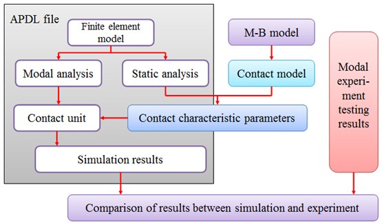
The finite model of the frame-shaped specimen considering the influence of the joint interface under uneven pressure was realised as follows: firstly, summation, clipping, and projection were carried out with HYPERMESH mesh generation so as to make all the unit nodes match one-to-one on the contact parts of the finite element model. Moreover, the nodes needed to be renumbered, thus constructing nodal sets with continuous serial numbers. Then, the pre-processed model was run through ANSYS software and a static analysis performed to find the pressure on each node under the effect of the pre-load. Afterwards, the pressures were introduced into the contact model program in MATLAB to calculate the stiffness and damping values of the nodes with those specific serial numbers. Finally, the units of stiffness and damping for the nodes and the node contact for the joint interface were established by using the matrix unit MATRIX27, and a finite element structural model, including the influence of the joint interface, was constituted.

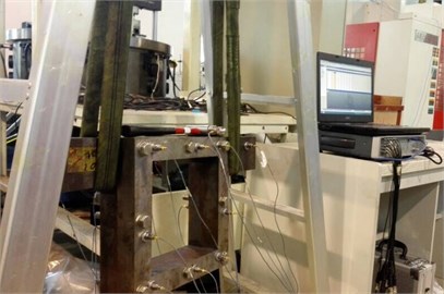
Aiming at the bolted joint parts of frame-shaped structural subassemblies, the hammering method was selected for the modal testing experiments in this study to obtain the dynamic characteristics, the inherent frequency, the vibration mode and the frequency response of the metal structure in the bolted joint parts. A knocking hammer equipped with a force sensor was used for the modal testing and analysis of the impact of the hammering method on the impulse-excited structure. The hammering point was located at Point 1, and the pretension force was selected to 9 kN, 12 kN and 15 kN, respectively. The specific sensor arrangement is shown in Fig. 6.

Fig. 6Illustration of the sensor arrangement

The inherent frequency and vibration mode of the structure basically determine the structural dynamics, and strongly depend on the contact rigidity at the joint interface. Thus, the accuracy of model can be validated by comparing the inherent frequency and vibration mode of the structure measured in the experiments with the corresponding values obtained through the simulation. A comparison of the simulation results is shown in Table 2.

Fig. 7Comparison of the results of the simulation and the experimental data for the deformation of a bolted joint interface

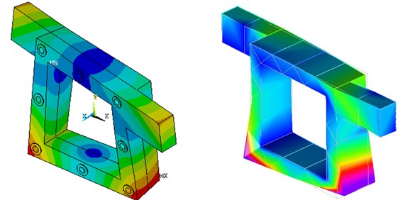
a) First-order deformation

b) Second-order deformation

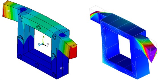
c) Third-order deformation

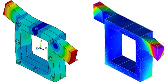
d) Fourth-order deformation

Table 2Comparison of the simulation results for the natural frequency of bolted joints under uniform load

	1st order	2nd order	3rd order	4th order	5th order	6th order
9 kN	549.74	625.6	821.13	840.55	1280.9	1463.1
12 kN	553.0	625.8	821.6	843.1	1282.2	1470.0
15 kN	555.26	625.92	821.88	844.73	1283.3	1474.5

For each order of the inherent frequency, the simulation results are in good agreement with the experimental results. The maximum error of 7.53 % was obtained for the 5th order inherent frequency under a uniform load of 15 kN. This is because the frame-shaped rack is not completely unrestrained, especially because the deformation mainly occurred on the beam where the ropes are attached, which will introduce a certain error. Meanwhile, the minimum error of 0.44 % was found for the 1st order inherent frequency under a uniform load of 15 kN All the errors are in an acceptable range. The results show that the contact rigidity model for the bolted joint interface can yield relatively accurate results for each order of the inherent frequency for different uniform loads. In order to more accurately verify the accuracy of the contact rigidity and damping model for a bolted joint interface, the theoretically and experimentally obtained principal vibration modes corresponding to each order of the inherent frequency are compared in Fig. 7. The results show that the simulation results are again in good agreement with the experimental results for each order of the principal vibration mode, which demonstrates the high accuracy of the contact rigidity model for the bolted joint interface, and the vibration-deformation of the joint part can be simulated with a high degree of accuracy.

To compare the simulated results with the vibration modes seen in the experiment, the centres of the adjacent sensor points arranged were used to construct correlation points by using LMS: then, all adjacent sensor points and correlation points were connected. Lastly, adjacent segments were used to form a polygon, which were further formed a plane through polygon filling. According to the results of the analysis, the simulation results under uneven pressure were superior to those under even pressure, which were closer to the experimental results, as shown in Fig. 7. Under the same conditions, the vibration modes and natural frequency were in the same order in both simulations and experiments: they were basically consistent. With increasing preload, the natural frequency, of the same order, increased, whereas the maximum vibration amplitude decreased (relatively). Moreover, the stiffness of the joint interface increased with increasing pre-load: both were quasi-linearly related.

According to formulae from Eqs. (20) to (46), the method can rapidly acquire the complex relationships among the contact parameters of a rough surface, and the normal force acting on the rough surface, the material properties parameters including: stiffness, yield strength, and equivalent elastic modulus, as well as the fractal dimension and fractal roughness of the rough surface. Among which, $D$ and $G$ can be obtained by using the prediction model. Afterwards, by using the model for predicting the surface morphology parameters in this study, an analysis of the structural properties of the joint interface can be realised by inputting an arbitrary processing parameter. Based on comparative tests and the natural frequencies and vibration modes of the joint interface, the precision of the contact model based on the improved deep neural network for predicting surface morphology parameters was verified.

6. Conclusions

1) In order to determine the influence of cold machining parameters on the surface appearance of rough surfaces, a surface appearance prediction model was established utilizing a regularized deep belief network. This model was demonstrated to effectively limit the overfitting problem and improve the accuracy of the prediction. The surface appearance parameters of the joint interface could be obtained by plugging arbitrary machining parameters into the model. Through training on the test samples and by comparing the measured values with the predicted values, the prediction model could predict the surface appearance parameters more accurately because the test data was provided by a high-precision topography instrument, and therefore a higher accuracy and a higher engineering value could be achieved.

2) The total and real contact area as well as the contact load of the joint interface were derived based on fractal theory and the Hertz contact theory. According to the definition of rigidity, a normal and a tangential contact rigidity model were established for the joint interface. Furthermore, according to the theory of energy consumption, the normal contact damping model was established based on the assumption that the energy consumption is related to the plastic deformation of the micro-bulges during the contact process. Meanwhile, the tangential contact damping model was established based on the assumption that the energy consumption can be attributed to friction in the micro-slip area of the micro-bulges.

3) The rigidity and damping matrixes of the joint interface were established in the FEM software using ANSYS and the Matlab software interface. Furthermore, frame-shaped test specimens were designed and built to represent the bolted joint parts of CNC machine tools. The simulation results were compared with experimental data for three different pretension forces, and the maximum error was found to be 7.53 %, which proves the reliability of the contact model proposed in this paper.

References

Ibrahim R. A., Pettit C. L. Uncertainties and dynamic problems of bolted joints and other fasteners. Journal of Sound and Vibration, Vol. 279, Issues 3-5, 2005, p. 857-936.

Publisher
Jiang Shu-yun, Zheng Yun-jian, Zhu Hua A contact stiffness model of machined plane joint based on fractal theory. ASME Journal of Tribology, Vol. 132, Issue 1, 2009, p. 1-7.

Publisher
Wen Shu-hua, Zhang Xue-liang, Wu Mei-xian, et al. Fractal model and simulation of normal contact stiffness of joint interfaces and its simulation. Transactions of the Chinese Society for Agricultural Machinery, Vol. 40, Issue 11, 2009, p. 197-202.

Search CrossRef
Greenwood J. A., Williamson J. B. P. Contact of nominally flat surfaces. Proceedings of the Royal Society of London. Series A. Mathematical and Physical Sciences, Vol. 295, Issue 1442, 1966, p. 300-319.

Publisher
Majumdar A., Bhushan B. Fractal model of elastic-plastic contact between rough surfaces. ASME Journal of Tribology, Vol. 113, Issue 1, 1991, p. 1-11.

Publisher
Zhang Xue-liang, Wang Nan-shan, Wen Shu-hua The elastic-plastic fractal model of energy dissipation for tangential contact damping of mechanical joint interface. Journal of Mechanical Engineering, Vol. 49, Issue 12, 2013, p. 43-49.

Publisher
Komvopoulos K., Ye N. Three-dimensional contact analysis of elastic-plastic layered media with fractal surface topographies. Journal of Tribology, Vol. 123, Issue 3, 2001, p. 632-640.

Publisher
Tian Hong-liang, Zhu Da-lin, Qin Hong-ling, et al. Modification of normal load’s analytic solutions for joint interface and quantitative experimental verification. Transactions of the Chinese Society for Agricultural Machinery, Vol. 42, Issue 9, 2011, p. 213-218.

Search CrossRef
Jiang S., Zhu H., Zheng Y. A contact stiffness model of machined plane joint based on fractal theory. Journal of Tribology, Vol. 132, Issue 1, 2010, p. 011401.

Search CrossRef
Yan W., Komvopoulos K. Contact analysis of elastic-plastic fractal surfaces. Journal of Applied Physics, Vol. 84, Issue 7, 1998, p. 3617-3624.

Publisher
Wen Shu-hua, Zhang Zong-yang, Zhang Xue-liang, et al. Stiffness fractal model for fixed joint interfaces. Transactions of the Chinese Society for Agricultural Machinery, Vol. 44, Issue 2, 2013, p. 255-260.

Search CrossRef
Liou J. L., Tsai C. M., Lin J. F. A microcontact model developed for sphere- and cylinder-based fractal bodies in contact with a rigid flat surface. Wear, Vol. 268, Issue 3, 2010, p. 431-442.

Publisher
Wang S. Development of theoretical contact width formulas and a numerical model for curved rough surfaces. Journal of Tribology, Vol. 129, Issue 4, 2007, p. 735-742.

Publisher
Bengio Y., Lamlin P., Popovici D., et al. Greedy layer-wise training of deep networks. Proceedings of Advances in Neural Information Processing Systems, 2007, p. 153-160.

Search CrossRef
Hinton G. E. Training products of experts by minimizing contrastive divergence. Neural Computation, Vol. 14, Issue 8, 2002, p. 1771-1800.

Publisher
Forsee F. D., Hagan F. D. Gauss-Newton approximation to Bayesian regularization. IEEE International Joint Conference on Neural Networks, Vol. 6, 1997, p. 1930-1935.

Search CrossRef
Pan G., Qiao J., Chai W., et al. An improved RBM based on Bayesian regularization. Neural Networks, Proceedings of the International Joint Conference on Neural Networks, 2014, p. 2935-2939.

Publisher
Cheng Lian-qing, Guo Jian-liang, Yang Xun, et al. Grinding roughness prediction model based on evolutionary artificial neural network. Computer Integrated Manufacturing Systems, Vol. 19, Issue 11, 2013, p. 2854-2863.

Search CrossRef
Zhao Hou-wei, Zhang Song, Zhao Bin, et al. Simulation and prediction of surface topography machined by ball-nose end mill. Computer Integrated Manufacturing Systems, Vol. 20, Issue 4, 2014, p. 880-889.

Search CrossRef
Kogut L., Etsion I. Elastic-plastic contact analysis of a sphere and a rigid flat. Journal of Applied Mechanics, Vol. 69, Issue 5, 2002, p. 657-662.

Publisher
Yan W., Komvopoulos K. Contact analysis of elastic-plastic fractal surfaces. Journal of Applied Physics, Vol. 84, Issue 7, 1998, p. 3617-3624.

Search CrossRef
Tian H. L., Zhao C. H., et al. Improved model of tangential stiffness for joint interface using anisotropic fractal theory. Transactions of the Chinese Society for Agricultural Machinery, Vol. 44, Issue 3, 2013, p. 257-266.

Search CrossRef
Zhang X., Wang N., Lan G., et al. Tangential damping and its dissipation factor models of joint interfaces based on fractal theory with simulations. Journal of Tribology, Vol. 136, Issue 1, 2014, p. 011704.

Publisher

Cited by

An Unsupervised Regularization and Dropout based Deep Neural Network and Its Application for Thermal Error Prediction

Yang Tian | Guangyuan Pan

(2020)

Systematic review of research relating to heavy-duty machine tool foundation systems

(2019)

Bearing deformation of heavy-duty machine tool-foundation systems and deformation detection methods

Yang Tian | Zhifeng Liu | Xiangmin Dong

(2019)

About this article

Received

02 September 2015

Accepted

08 January 2016

Published

15 May 2016

SUBJECTS

Mechanical vibrations and applications

DOI

https://doi.org/10.21595/jve.2016.16373

Keywords

regularization

deep belief network

fractal theory

joint interface

Acknowledgements

This work was supported by National Science and Technology Major Project (2013ZX04013011), Jing-Hua Talents Project of Beijing University of Technology, the National Natural Science Foundation of China (51575009), the Beijing Natural Science Fund (3162003) and the Science Research General Project of Liaoning Province Education Department (L2014589).

This is an open access article distributed under the Creative Commons Attribution License, which permits unrestricted use, distribution, and reproduction in any medium, provided the original work is properly cited.

Next article in issue Next

Review article

2023 11 04

A comprehensive review of mechanical fault diagnosis methods based on convolutional neural network

Junjian Hou, Xikang Lu, Yudong Zhong, Wenbin He, Dengfeng Zhao, Fang Zhou

Research article

2023 08 01

A fault diagnosis method based on dilated convolution and attention for rolling bearing under multiple working conditions and noisy environments

Hui Zhang, Shengdong Liu, Ziwei Lv, Zhenlong Sang, Fangning Li

Research article

2023 04 13

Diagnosis of rotating machinery based on improved convolutional neural networks with gray-level transformation

Guofang Nan, Jianwei Wang, Di Ding

Review article

2021 11 26

Fault diagnosis and health management of bearings in rotating equipment based on vibration analysis – a review

Adnan Althubaiti, Faris Elasha, Joao Amaral Teixeira

Y. Tian, Z. Liu, L. Cai, and G. Pan, “The contact mode of a joint interface based on improved deep neural networks and its application in vibration analysis,” Journal of Vibroengineering, Vol. 18, No. 3, pp. 1388–1405, May 2016, https://doi.org/10.21595/jve.2016.16373

Copy Extrica

Copied to clipboard!

TY  - JOUR
DO  - 10.21595/jve.2016.16373
UR  - https://doi.org/10.21595/jve.2016.16373
TI  - The contact mode of a joint interface based on improved deep neural networks and its application in vibration analysis
T2  - Journal of Vibroengineering
AU  - Liu, Zhifeng
AU  - Tian, Yang
AU  - Cai, Ligang
AU  - Pan, Guangyuan
PY  - 2016
DA  - 2016/05/15
PB  - JVE International Ltd.
SP  - 1388-1405
IS  - 3
VL  - 18
SN  - 1392-8716
ER  - 

Copy Ris

Copied to clipboard!

@article{Liu_2016,
	doi = {10.21595/jve.2016.16373},
	url = {https://doi.org/10.21595/jve.2016.16373},
	year = 2016,
	month = {may},
	publisher = {{JVE} International Ltd.},
	volume = {18},
	number = {3},
	pages = {1388--1405},
	author = {Zhifeng Liu and Yang Tian and Ligang Cai and Guangyuan Pan},
	title = {The contact mode of a joint interface based on improved deep neural networks and its application in vibration analysis},
	journal = {Journal of Vibroengineering}
}

Copy Bibtex

Copied to clipboard!

[1]Z. Liu, Y. Tian, L. Cai, and G. Pan, “The contact mode of a joint interface based on improved deep neural networks and its application in vibration analysis,” Journal of Vibroengineering, vol. 18, no. 3, pp. 1388–1405, May 2016, doi: 10.21595/jve.2016.16373.

Copy IEEE

Copied to clipboard!

Liu, Zhifeng, Yang Tian, Ligang Cai, and Guangyuan Pan. “The Contact Mode of a Joint Interface Based on Improved Deep Neural Networks and Its Application in Vibration Analysis.” Journal of Vibroengineering 18, no. 3 (May 15, 2016): 1388–1405. https://doi.org/10.21595/jve.2016.16373.

Copy Chicago

Copied to clipboard!

The contact mode of a joint interface based on improved deep neural networks and its application in vibration analysis

Abstract

1. Introduction

2. Regularized deep belief network model

2.1. Structure of the neural network

2.2. The neural network algorithm

3. Application of the prediction model

3.1. Training samples

3.2. Experimental results

4. Contact model

4.1. The real contact area model for the joint interface

4.2. Normal contact rigidity model for the joint interface

4.3. Tangential contact rigidity model for a joint interface

4.4. Normal contact damping model for a joint interface

4.5. Tangential contact damping model for the joint interface

5. Experimental analysis

6. Conclusions

References

Cited by

About this article

Related Articles