Sliding mode force tracking control for active hydro-pneumatic suspension

Guan, Jifu; Huo, Dongdong; Ji, Xinxia

Journal of Vibroengineering

Browse Journal

Submit article

Published: 15 February 2016

Check for updates

Sliding mode force tracking control for active hydro-pneumatic suspension

Jifu Guan¹

Dongdong Huo²

Xinxia Ji³

^{1, 2, 3}Laboratory of Vibration and Noise Control, Beijing Institute of Technology, Beijing, 100081, China

Corresponding Author:

Jifu Guan

Cite the article Download PDF

Downloads 1206

Abstract

A nonlinear state equation model of Active Hydro-Pneumatic suspension (AHP) system is established basing on power bond graph theory. The nonlinear characteristics of stiffness and friction of the hydro-pneumatic spring actuator and the oil compressibility are considered in modeling. Meanwhile, a theoretical analysis is conducted for dynamic structural characteristics of hydro-pneumatic spring actuator. A sliding mode control (SMC) strategy is presented which has two closed-loops, where the outer loop considers the sprung velocity of skyhook reference model output as tracking target and the inner loop regards the desired force of the sliding mode solver as tracking target. Simultaneously, the sliding mode control laws of inner and outer loops are deduced. Especially, a divergence problem of outer loop sliding model solver caused by time delay is analyzed and a stabilization control algorithm is put forward to solve it. The accurate tracking of desired force of actuator and the improvement of ride quality are realized, while the effectiveness of the proposed sliding mode control law and stabilization control algorithm are verified through simulation studies of relevant contrast test.

1. Introduction

The concept of active suspension refers that there is a controllable force between sprung mass and unsprung mass. So the previous works of concerning control algorithm were mainly based on linear model to get the control law of optimal control force, not considering the structure principles and dynamic characteristics of the actuator which produces control force [1]. In recent years, with the development of active suspension rig experiment, people pay more attention to the generated mechanism of control force and the dynamic characteristics of actuator which have significant influences on the system control performance and become a crucial factor restricting active suspension engineering realization [2].

Alleyne [3-6] established a suspension nonlinear model comprising the actuators’ dynamics, in which the actuator is a controlled hydraulic cylinder. And he proposed a sliding force tracking control taking the skyhook model output as the desired force. He also revealed challenges of achieving force tracking control due to a negative feedback of relative velocity existing in the actuator dynamics model. Since that the following pertinent literature [7-11] which researched nonlinear control algorithm of force tracking mostly adopted the actuator dynamics model proposed by Alleyne. However, the scheme of hydraulic cylinder actuator proposed by Alleyne required the suspension being in active state. If stop charging or discharging oil control, the suspension will be locked in a rigid state and the suspension system will lose damping effect. For these reasons, the scheme of hydraulic cylinder actuator would be difficult to apply in engineering.

However, the active suspension system taking a controlled charge and discharge of hydro-pneumatic springs as actuators has higher practicability due to it switching between active suspension and passive suspension. But the dynamic characteristics of hydro-pneumatic spring actuator is different from the traditional hydraulic cylinder actuator proposed by Alleyne owing to the oil and gas coupling, nonlinear stiffness and other factors in the process of charging and discharging oil of hydro-pneumatic spring actuator, therefore to realize force tracking control for hydro-pneumatic spring actuator has more difficulties compared to the traditional hydraulic cylinder actuator. The research on control of active hydro-pneumatic suspension including dynamic characteristics of hydro-pneumatic spring actuator is still not enough at present. M. D. Emami [12] established bond graph model of active hydro-pneumatic suspension system and studied its dynamics based on this model. J-W Shi [13] proposed a new linearization method for hydro-pneumatic suspension system basing on its affine nonlinear characteristics. Mehmet Akar [14] achieved the body height control of vehicle with two closed-loops control strategy, where the inner loop is sliding force tracking control and the outer loop is PID control.

This paper aims at researching on sliding force tracking control of hydro-pneumatic suspension basing on the background of an engineering project about AHP system. It is organized as follows. Section 2 briefly outlines the schematic of AHP system and skyhook structure. Section 3 sheds light on the detail process of modeling about AHP system. The dynamic characteristics of electro-hydraulic proportional valve, nonlinear stiffness characteristics, friction nonlinear characteristics, and the oil compressibility caused by mixing oil and gas in engineering are taken into account in modeling process of AHP. The power bond graph theory is employed to create the nonlinear models of state space equation of AHP and skyhook systems, and the simulation parameters are listed. Section 4 deduces the hydro-pneumatic spring actuator’s dynamics and analyzes generation mechanisms of control force and difficulties of force tracking control faced. Section 5 presents a double closed-loop sliding mode control strategy which takes the skyhook model’s relative velocity output as outer loop tracking target and regards the desired pressure of oil chamber of actuator as the inner loop tracking target, then deduces a sliding mode control law of outer loop which named sliding mode solver and inner loop which named sliding mode controller, especially a divergence problem of outer loop’s sliding mode solver caused by time delay is analyzed and a stabilization control algorithm is put forward to deal with it. Section 6 conducts a systematical simulation and theoretical analysis. The accurate tracking of desired force of actuator and the improvement of ride comfort are realized, while the effectiveness of the proposed sliding mode control law and stabilization control algorithm are verified through simulation studies of relevant contrast test.

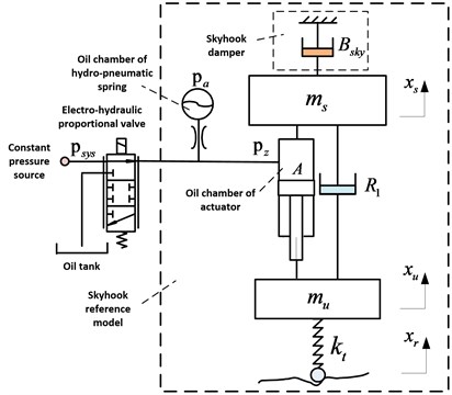
2. Active hydro-pneumatic suspension system schematic

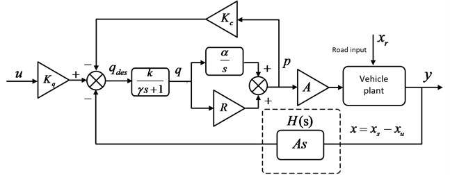
Active hydro-pneumatic suspension (AHP) and skyhook reference system are shown in Fig. 1. Where, the schematic inside the dashed box is the skyhook reference system. Without the skyhook damper, the remained part is the AHP system. AHP is composed by electro-hydraulic proportional servo valve, hydro-pneumatic spring, actuator, oil source and so on. The fluid flow of charge or discharge can be adjusted through control of displacement of servo spool valve. Specially, the suspension is in a passive state when the servo valve is closed.

3. Active hydro-pneumatic suspension model

3.1. Electro-hydraulic proportional servo valve

Suppose $Q_{v}$ as the output flow of electro-hydraulic proportional servo valve, $I$ as the control current, $I_{m a x}$ as the maximum control current, $p_{z}$ as the oil chamber pressure of actuator, $p_{s y s}$ as the pressure of constant pressure source. When hydraulic fluid flow through orifice of the servo valve, the relationship between the control current $I$ of servo valve and fluid flow $Q_{v}$ is given as follows:

1

Q_{v} (I, p_{Z}) = K_{v} S a t (\frac{I}{I_{m a x}}) \sqrt{p_{s} - p_{z} s g n (I)},

2

p_{s} = \{\begin{array}{l} I \geq 0, p_{s y s}, \\ I < 0, 0, \end{array} S a t (\frac{I}{I_{m a x}}) = \{\begin{array}{l} I, I \leq I_{m a x}, \\ s g n (\frac{I}{I_{m a x}}), I > I_{m a x} . \end{array}

Fig. 1AHP and skyhook reference system

3.2. Hydro-pneumatic spring

Assume that the work process of hydro-pneumatic spring is an adiabatic process, the gas polytropic index is $γ$ , initial pressure and volume is $p_{g 0}$ and $V_{g 0}$ respectively, $p_{a}$ is the pressure of hydro-pneumatic spring, $K_{a}$ is stiffness of hydro-pneumatic spring, $V_{a}$ is the compression volume of hydro-pneumatic spring relative to $V_{g 0}$ . Thus the nonlinear properties of pressure and stiffness of hydro-pneumatic spring are given as follows and shown in Fig. 2.

Pressure properties:

3

p_{a} = {ϕ_{c}}^{- 1} (V_{a}) = p_{g 0} {(\frac{V_{g 0}}{V_{g 0} - V_{a}})}^{γ} .

Stiffness properties:

4

K_{a} = \frac{γ p_{g 0} {V_{g 0}}^{^{γ}}}{{(V_{g 0} - V_{a})}^{γ + 1}} .

Fig. 2The nonlinear properties of pressure and stiffness

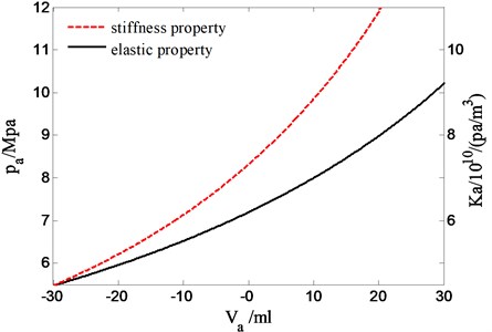
As shown in Fig. 2, $V_{a}$ is used as the abscissa to describe the pressure and stiffness properties of hydro-pneumatic spring. In this figure, the solid line and the coordinate on left side of the line indicate the pressure properties represented by the Eq. (3), besides the dotted line and the coordinate on right side of the line indicate the stiffness properties represented by the Eq. (4).

Considering the hydro-pneumatic spring is filled with nitrogen, whose working process satisfies a polytropic process and the gas in this process is jointly determined by the initial state $p_{g 0}$ , $V_{g 0}$ and the polytropic exponent $γ$ . The initial pressure and volume of the hydro-pneumatic spring is the actual object of the research process. The working process of hydro-pneumatic spring is a polytropic process between isothermal process and adiabatic process, which polytropic exponent shows a certain trend when taking into the influence of environment and complex factors account. With the overall consideration, the value of $γ$ is taken as 1.25 by referring to the actual experimental data and research simplifying.

3.3. Damping characteristics of pipeline

As shown in Fig. 1, the fluid resistance of main pipeline can be equivalent into suspension damping. Provided that $p_{a}$ is the oil chamber pressure of hydro-pneumatic spring, $p_{z}$ is the oil chamber pressure of actuator, $R$ is the pipeline damping of hydro-pneumatic spring. So the damping characteristics of pipeline are:

5

q = \frac{p_{z} - p_{a}}{R} .

3.4. The oil compressibility

Suppose that the oil volume is $V$ , initial pressure is $p$ , elastic modulus is $β$ . From the definition of the elastic modulus, we can know that the compressibility of given oil quality satisfies following relationship [15]:

6

β = - \frac{d p}{d V} V .

The oil pressure will change when fill the oil into a container which volume is variable. Assume that initial volume and pressure of container is $V_{0}$ and $p_{0}$ respectively. Within the time $d t$ , the pressure changes $d p$ and the oil volume filled in container is $d V_{i n}$ . Suppose the being compressed oil volume is positive, so the amount of change in the volume of the container is:

7

d V = - V_{0} \frac{d p}{β} + d V_{i n} .

Let:

8

d V_{o p} = V_{0} \frac{d p}{β} .

Take the initial volume of oil chamber as the foundation and equal to elastic component, $V_{0}$ represents the initial volume of the oil chamber of hydro-pneumatic spring. According to the Eq. (8), we can get that the oil compression flow of the oil chamber of hydro-pneumatic spring $q_{o}$ is:

9

q_{o} = \frac{V_{0}}{β} \dot{p} = \frac{V_{0}}{β} K_{a} q_{a} = h (V_{a}) q_{a},

where, $h (V_{a}) = \frac{V_{0}}{β} K_{a}$ .

3.5. Friction characteristics

We use a friction model which is composed by a smooth continuous arc tan function in case that the singularity appears in the derivation to make the simulation of system convenient. Suppose $v$ is the relative velocity, $F_{C}$ , $F_{m}$ , $c_{0}$ , $k_{1}$ and $k_{2}$ are parameters of friction. Thus the friction of actuator is defined as follows [16]:

10

F_{f} = R_{2} (v) = - F_{C} \frac{2 t a n^{- 1} (- k_{1} v)}{π} - F_{m} \frac{2 t a n^{- 1} (- k_{2} v)}{π} + c_{0} v .

Define the coulomb friction as follows:

F_{d} = - F_{C} \frac{2 t a n^{- 1} (- k_{1} v)}{π} - F_{m} \frac{2 t a n^{- 1} (- k_{2} v)}{π} .

$F_{d}$ derivation of the speed is as following:

{\dot{F}}_{d} = \frac{2 k_{1} F_{C}}{π + π k_{1}^{2} {v_{s}}^{2}} + \frac{2 k_{2} F_{m}}{π + π k_{2}^{2} {v_{s}}^{2}} .

Set ${\dot{F}}_{d}$ , critical speed $V_{s}$ and static friction force $F_{s}$ can be obtained:

11

v_{S} = \sqrt{- \frac{k_{2} F_{m} + k_{1} F_{C}}{{k_{1}}^{2} k_{2} F_{m} + {k_{2}}^{2} k_{1} F_{C}}} = 4 mm / s,

12

F_{S} = - F_{C} \frac{2 t a n^{- 1} (- k_{1} v_{S})}{π} - F_{m} \frac{2 t a n^{- 1} (- k_{2} v_{S})}{π} = 128 N .

When the speed tends to $\infty$ , the Coulomb friction $F_{C O}$ could be get:

13

F_{C O} = F_{C} - F_{m} = 53 N .

When $v = 0$ , the maximum static friction force $F_{s}$ can be acquired by selecting the appropriate speed stiffness ${\dot{F}}_{d} (0)$ :

14

{\dot{F}}_{d} (0) = \frac{2 k_{1} F_{C}}{π} + \frac{2 k_{2} F_{m}}{π} = 1.85 e 5 N /(m / s)

So according to the Eqs. (11)-(14), the physical processes of dynamic transformation from static friction force to Coulomb friction can be obtained by selecting appropriate $F_{C}$ , $F_{m}$ , $c_{0}$ , $k_{1}$ and $k_{2}$ , and it is shown in Fig. 3.

4. Active hydro-pneumatic suspension bond graph model

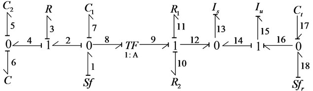
According to the analysis above, we can get the bond graph model of AHP shown in Fig. 4.

Where, flow sources $S f$ and $S f_{r}$ is the flow input of proportional electro-hydraulic servo valve and velocity input of road excitation respectively, and $C$ , $C_{1}$ , $C_{2}$ , $C_{t}$ separately represents the elasticity of hydro-pneumatic spring, oil chamber of hydro-pneumatic spring, oil chamber of actuator and the tire, and $R$ , $R_{1}$ , $R_{2}$ separately represents oil damping of hydro-pneumatic spring, suspension damping and actuator friction, and $I_{s}$ , $I_{u}$ separately represents suspension sprung and unsprung mass.

Choose $q_{6}$ , $e_{7}$ , $p_{13}$ , $p_{15}$ , $q_{17}$ as the system state variables. The initial value of System state variables is all zero. These symbols are symbolic notation of power bond graph.

Set:

x = {[\begin{array}{l} \frac{p_{13}}{I_{s}} & e_{7} + p_{g 0} & q_{6} & \frac{p_{15}}{I_{u}} & q_{17} \end{array}]}^{T} .

Fig. 3Friction model

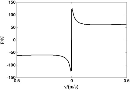
Fig. 4Bond graph model of AHP

Then the state equation of the system is:

\{\begin{array}{l} {\dot{x}}_{1} = \frac{1}{I_{s}} (A (x_{2} - p_{g 0}) - R_{1} (x_{1} - x_{4}) - R_{2} (x_{1} - x_{4})), \\ {\dot{x}}_{2} = \frac{β}{V_{c}} (Q_{v} (I, x_{2}) - \frac{x_{2} - {ϕ_{c}}^{- 1} (x_{3})}{R} - A (x_{1} - x_{4})), \\ {\dot{x}}_{3} = \frac{x_{2} - {ϕ_{c}}^{- 1} (x_{3})}{(1 + h (x_{3})) R}, \\ {\dot{x}}_{4} = - \frac{1}{I_{u}} (\frac{x_{5}}{C_{r}} + A (x_{2} - p_{g 0}) - R_{1} (x_{1} - x_{4}) - R_{2} (x_{1} - x_{4})), \\ {\dot{x}}_{5} = x_{4} - S f_{r} . \end{array}

4.1. Skyhook reference model

Relative to passive suspension, skyhook model can effectively improve the ride quality in the range of resonance point of sprung mass. So taking skyhook model as reference model to get force tracking control of suspension system can effectively improve the suspension ride quality. Skyhook reference model state variable is set as $x_{r}$ and its state equation is rewritten as follows:

\{\begin{array}{l} {\dot{x}}_{r 1} = \frac{1}{I_{s}} (A (x_{r 2} - p_{g 0}) - R_{1} (x_{r 1} - x_{r 4}) - R_{2} (x_{r 1} - x_{r 4}) - B_{s k y} x_{r 1}), \\ {\dot{x}}_{r 2} = - \frac{β}{V_{c}} (\frac{x_{r 2} - {ϕ_{c}}^{- 1} (x_{r 3})}{R} + A (x_{r 1} - x_{r 4})), \\ {\dot{x}}_{r 3} = \frac{x_{r 2} - {ϕ_{c}}^{- 1} (x_{r 3})}{(1 + h (x_{3})) R}, \\ {\dot{x}}_{r 4} = - \frac{1}{I_{u}} (\frac{x_{r 5}}{C_{r}} + A (x_{r 2} - p_{g 0}) - R_{1} (x_{r 1} - x_{r 4}) - R_{2} (x_{r 1} - x_{r 4})), \\ {\dot{x}}_{r 5} = x_{r 4} - S f_{r} . \end{array}

Desired pressure force:

15

p_{d e s} = x_{r 2} - \frac{B_{s k y}}{A} x_{r 1} .

4.2. System simulation parameters

The simulation parameters are listed on Table 1.

Table 1Simulation parameters

Parameters	Value
Servo valve coefficient $K_{v}$	6 e-7
Maximum input current $I_{m a x}$ / A	2
Oil supply pressure $P_{s y s}$ / MPa	10
The initial volume of hydro-pneumatic spring $V_{g 0}$ / ml	100
The initial pressure of hydro-pneumatic spring $p_{g 0}$ / MPa	7.31
Gas polytropic index $γ$	1.25
Pipeline damping $R$ / (Pa/(m³/s))	2.08 e9
Oil elastic modulus $β$ / MPa	1000
The initial volume of the oil chamber of hydro-pneumatic spring $V_{o}$ / ml	60
The initial volume of actuator $V_{c}$ / ml	90
Actuator piston area $A$ / m³	8.2 e-4
Friction parameter $F_{C}$ / N	153
Friction parameter $F_{m}$ / N	100
Friction parameter $c_{0}$ / (N/(m/s))	20
Friction parameter $k_{1}$ / (N/(m/s))	1937
Friction parameter $k_{2}$ / (m/s)	–50
Suspension damping $R_{1}$ / (N/(m/s))	2500
Sprung mass $I_{s}$ / kg	612
Unsprung mass $I_{u}$ / kg	80
Tire flexibility $C_{t}$ / (m/N)	5.38 e-6

5. Actuator dynamics

By the state equation of the system, we can obtain that:

16

{\dot{p}}_{z} = \frac{β}{V_{c}} (Q_{v} (I, p_{z}) - \frac{p_{z} - {ϕ_{c}}^{- 1} (V_{a})}{R} - A \dot{x}) .

Conduct a linearization process for the Eqs. (5), (9), (12). We can get that:

17

\frac{V_{c}}{β} s p_{z} + q = K_{q} I - K_{c} p - A s x,

18

R q = p_{z} - K_{a} \frac{β}{β + V_{0} K_{a}} q \frac{1}{s} .

Set:

α = \frac{β K_{a}}{β + V_{0} K_{a}}, γ = \frac{V_{c} R}{V_{c} α + β}, k = \frac{β}{V_{c} α + β}, q_{d e s} = K_{q} I - K_{c} p - A s x .

So according to Eq. (17), (18) we can obtain:

19

p_{z} = R q + α q \frac{1}{s},

20

q = \frac{k}{γ s + 1} q_{d e s} .

Therefore, we can acquire the dynamic model of hydro-pneumatic spring actuator shown in Fig. 5.

Fig. 5The dynamic model of hydro-pneumatic spring actuator

We can know from the Fig. 5 that it exists the conclusion similar to Y. Zhang [6]. Due to the presence of negative feedback term which is the cylinder relative velocity, it makes the poles of the vehicle plant become the zero of open-loop force transfer function. If these zeros are lightly damped or undamped, the achievable bandwidth of any controller will be limited. Therefore, to realize the force tracking control for active suspension system comprising hydraulic actuator will face serious challenges. The difference between the actuator of hydro-pneumatic spring and the actuator that Y. Zhang studied is the generation mechanism of actuator’s output force. Hydro-pneumatic suspension actuator’s output force not only depends on the pressure of the oil chamber of actuator but also relies on the pressure variation of the oil chamber of hydro-pneumatic spring. Because inertial element formed by oil compressibility and pipeline damping causes a delay to the response of oil flow of hydro-pneumatic spring pipeline. Only when the oil is incompressible or the pipeline damping does not exist, the impact on the hydro-pneumatic suspension force tracking control resulting from the negative feedback segment will be perfectly canceled. The output force of actuator is achieved mainly through integration accumulating in time for the pipeline flow. So this also poses a challenge to the response of output force tracking of actuator.

6. Sliding mode control

Sliding mode control is a robust control strategy applied to uncertain nonlinear systems. Its convergence is decided by time varying sliding surface. When the model error is zero, the system will eventually keep on the sliding surface under the inputs drive. When the model exists uncertainties, the system will eventually converge to the boundary layer of the sliding surface. Sliding mode control law generally constitutes by the continuous control item and switching control item [17].

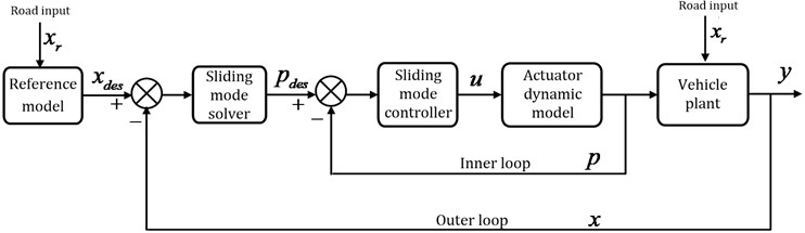
6.1. Force tracking control structure

Fig. 6 is the force tracking control structure diagram. The outer loop tracks desired state variable of system, which is the absolute velocity of sprung mass output by skyhook reference model, and the desired tracking force tracked by inner loop is calculated by sliding mode solver. The inner loop is constituted by a sliding mode controller. Therefore, the force tracking control structure presented in this paper may achieve the improvement of suspension ride quality.

Fig. 6Force tracking control structure

6.2. Sliding mode controller and solver design

Define:

u_{1} = x_{2}, g_{1} = \frac{A}{I_{s}}, x = x_{1} - x_{4}, f_{1} (x) = - \frac{1}{I_{s}} (A p_{g 0} + R_{1} (x_{1} - x_{4}) + R_{2} (x_{1} - x_{4})) .

So the sprung velocity satisfies the following relationship:

21

{\dot{x}}_{1} = f_{1} (x) + g_{1} u_{1} .

Define:

u_{2} = I, g_{1} (x) = \frac{β K_{v}}{V_{c}} \sqrt{P_{s} - x_{2} s g n (I)}, f_{2} (x) = - \frac{β (x_{2} - {ϕ_{c}}^{- 1} (x_{1}))}{R V_{c}} - \frac{A β}{V_{c}} (x_{1} - x_{4}) .

The flow balance relationship of hydro-pneumatic suspension is as follows:

22

{\dot{x}}_{2} = f_{2} (x) + g_{2} (x) u_{2} .

Set $i =$ 1, 2, so we can get:

23

{\dot{x}}_{i} = f_{i} (x) + g_{i} (x) u_{i} .

Due to the parameters of $f_{i} (x)$ and $g_{i} (x)$ have uncertainties and exist unmodeled dynamics, we suppose the uncertain boundary is:

24

|f_{i} (x) - {\hat{f}}_{i} (x)| \leq F_{i},

25

0 < g_{i m i n} \leq {\hat{g}}_{i} (x) \leq {g_{i}}_{m a x} .

Use geometric average as the estimation of $g_{i} (x)$ :

26

{\hat{g}}_{i} = \sqrt{{g_{i}}_{m a x} {g_{i}}_{m i n}} .

Defined sprung velocity tracking error and force tracking error are:

27

ε_{i} = x_{i} - x_{i d e s} .

Sliding surface is defined as follows[18]:

28

s_{i} = (\frac{d}{d t} + λ_{i}) (\int_{0}^{t} ε_{i} d t) = ε_{i} + λ_{i} \int_{0}^{t} ε_{i} d t .

Sliding surface convergence conditions is:

29

{\dot{s}}_{i} = - η_{i} s_{i} .

According to Eq. (25), (29), (31), we get:

30

{\hat{u}}_{i} = {\hat{g}}_{i} (x)^{- 1} (- f_{i} (x) + {\dot{x}}_{i d e s} - (λ_{i} + η_{i}) ε_{i} - η_{i} λ_{i} \int_{0}^{t} ε_{i} d t) .

Switch control item:

31

u_{i p} = - {\hat{g}}_{i} (x)^{- 1} k_{i} s g n (s_{i}) .

The gain $k_{i}$ satisfies the following relationship:

32

k_{i} \geq α_{i} (F_{i} + η_{i}) + (α_{i} - 1) |{\hat{g}}_{i} {\hat{u}}_{i}|,

33

α_{i} = \sqrt{\frac{g_{i m a x}}{g_{i m i n}}} .

So the sliding mode solver and controller are as follows:

34

u_{i} = {\hat{g}}_{i} (x)^{- 1} (- f_{i} (x) + {\dot{x}}_{i d e s} - (λ_{i} + η_{i}) ε_{i} - η_{i} λ_{i} \int_{0}^{t} ε_{i} d t - k_{i} s g n (s_{i})) .

6.3. Controller parameters

The model uncertain boundary error is in the twenty percent range:

35

F_{i} = 0.2 {\hat{f}}_{i} (x),

36

{g_{1}}_{m a x} = \frac{1}{1.2} g_{1}, {g_{1}}_{m i n} = \frac{1}{0.8} g_{1},

37

{g_{2}}_{m a x} = 1.2 g_{2}, {g_{2}}_{m i n} = 0.8 g_{2} .

The parameters’ value of sliding mode controller and solver are given as follows:

η_{1} = 0.1, λ_{1} = 0.1, η_{2} = 1 e 4, λ_{2} = 5 e 3 .

6.4. Controller delay stabilization

Suppose existing time delay $τ$ , define operation:

38

δ e = e (t) - e (t - τ) .

Eq. (38) reflects the disturbances of signal $e$ under the circumstance of time difference $τ$ . We do decomposition for the linear and nonlinear term of Eq. (19) and get:

39

{\dot{x}}_{i} = - A_{i} x_{i} + h_{i} (x) + g_{i} (x) u_{i},

where, $h_{i} (x)$ represents the nonlinear term.

According to Eqs. (38), (39), we can get:

40

δ {\dot{x}}_{i} = - A_{i} δ x_{i} + δ h_{i} (x) + δ (g_{i} (x) u_{i}) .

Eq. (40) is a system dynamic reflecting the disturbance of system state. Obviously in order to achieve the smooth tracking for desired signal, controllers should have ability to quickly restrain such disturbance.

Assume existing inequalities:

‖δ h (x)‖ \leq δ h_{0}, ‖g_{i} (x)‖ \leq B_{i} .

Then we can get [17]:

41

‖δ x_{i}‖ \leq ‖δ x_{i} (t_{0})‖ e^{- A_{i} τ} + \frac{1}{A_{i}} (B_{i} \underset{t_{0} \leq t \leq t_{n}}{s u p} ‖δ u_{i} (t_{0})‖ + δ h_{0}) .

From the Eq. (41), we can get that $A_{i}$ reflects the restrain level of system to disturbance. In order to make the response of state caused by disturbance quickly decay, $A_{i}$ must be large enough.

From the Eq. (40), we can get: $A_{1} = 4.12$ , $A_{2} = 5342$ .

Obviously it need to stabilize the sliding mode solver to make system achieve a quickly suppression to the disturbance. The solver dynamic process is as follows:

42

u_{1} = {\hat{g}}_{1}^{- 1} (- f_{1} (x (t - τ)) + {\dot{x}}_{1 d e s} - λ_{1} ε_{1} - η_{1} s - k_{1} s g n (s_{1})) .

Tire deformation is assumed as $w,$ suspension relative velocity satisfies the following relationship:

43

\dot{x} = (\frac{1}{I_{s}} + \frac{1}{I_{u}}) (A u_{1} + I_{s} f_{1} (x (t))) + \frac{k_{t}}{I_{u}} w .

Suppose:

f (x) = - \frac{I_{s} + I_{u}}{I_{u}} f_{1} (x (t)) .

So $f (0) = 0$ , $f (x)$ is a monotone increasing function.

Suppose:

I = \frac{I_{s} + I_{u}}{I_{u}} ({\dot{x}}_{1 d e s} - λ_{1} ε_{1} - η_{1} s - k_{1} s g n (s_{1})) + \frac{k_{t}}{I_{u}} w .

According to Eqs. (42), (43), we can know that relative velocity has the following form:

44

\dot{x} = - δ f (x) + I .

Set:

δ (δ f (x)) = δ^{2} f (x) .

According to Eqs. (38), (44), we can get:

45

δ \dot{x} = - δ^{2} f (x) + δ I .

$δ^{2} f (x)$ is a higher-order disturbance term, obviously $δ^{2} f (x)$ has little influence on the input disturbance $δ I$ . Now consider adding disturbance restrain item:

46

δ \dot{x} = - μ δ x - δ^{2} f (x) + δ I .

Suppose existing:

‖δ^{2} f (x)‖ \leq δ^{2} f_{0} .

So we can get [17]:

47

‖δ x‖ \leq ‖δ x (t_{0})‖ e^{- μ τ} + \frac{1}{μ} (\underset{t_{0} \leq t \leq t_{n}}{s u p} ‖δ I‖ - δ^{2} f_{0}) .

Obviously by designing an appropriate $μ$ value, we can achieve effective suppress to the disturbance. Then through stabilization, relative velocity has the following form:

48

\dot{x} = - μ x - δ f (x) + I .

Owing to $τ$ is very small, so there is:

49

x (t) \approx x (t - τ) .

According to Eqs. (43), (48), (49), we can get the final equation of solver:

50

u_{1} = {\hat{g}}_{1}^{- 1} (- μ x - f_{1} (x) + {\dot{x}}_{1 d e s} - λ_{1} ε_{1} - η_{1} s - k_{1} s g n (s_{1})) .

From Eqs. (21), (28), (50), we can get:

51

\dot{s} + η_{1} s = μ x - k s g n (s) .

So we obtain [17]:

52

‖s‖ \leq ‖s_{0}‖ e^{- η t} + \frac{μ * \underset{t_{0} \leq τ \leq t}{s u p} ‖x‖ + k}{η} .

According to Eqs. (46), (47), (52), we can deduce that $μ$ effects the restrain level of disturbance to $x$ . At the same time, it also affects the sliding boundary layer. The lager $μ$ is, the smaller the disturbance range of relative velocity is, vice versa. Therefore, there is an optimal $μ$ value making the sliding boundary layer minimum, in the following simulation, $μ =$ 250.

7. Simulation and analysis

The nonlinear model of active hydro-pneumatic suspension is established in Matlab/Simulink to verify the proposed sliding mode control algorithm. The following section is divided into three parts to introduce the results of the simulation. Part1 shows the effectiveness of time delay stabilization algorithm through unstabilized and stabilized comparison. Part 2 depicts the tracking effects of inner loop for a desired force, and makes a contrast with the effectiveness of PID, as a result, the improvement of acceleration of sprung mass is also illustrated. Part 3 gives the simulation results of sprung velocity tracking for a stochastic road input to verify the stability and effectiveness of the proposed double-loop sliding control system, meanwhile, the percentage of improvement of sprung acceleration and the tracking error of sprung velocity are calculated respectively for the tracking of desired force and tracking desired velocity, which are the output of skyhook. Part 3 also shows the result of body displacement as the potential ability of proposed algorithm due to the integration form utilizing in sliding mode solver.

7.1. Time delay stabilization simulation

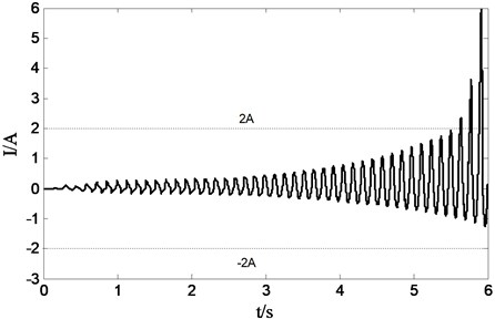
Figs. 7 and 8 reflect the situation of sliding mode solver tracking the sprung velocity when system is unstabilized. It is shown that the tracking error of sprung velocity is continuous increasing in Fig. 7 due to the system itself weak in restraining disturbance, especially the tracking deviation of sprung velocity becomes more apparently owing to the saturation limitation of current when the amplitude of current signal is greater than 2 $A$ in Fig. 8.

Fig. 7The sprung velocity tracking

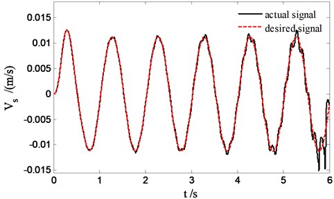
Fig. 8Current signal

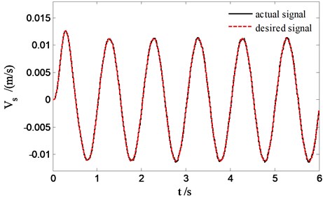
It is shown in Fig. 9 that the actual sprung velocity signal accurately tracks the desired sprung velocity because of the stabilization of sliding mode solver manifesting the effectiveness of the presented algorithm in this paper.

Fig. 9The velocity tracking of sprung mass

7.2. Force tracking control effect

Fig. 10 indicates the force tracking effect to desired pressure $p_{d e s}$ of skyhook reference model output with PID controller instead of the sliding mode controller. It is shown that for PID controller conducting force tracking, there is a phase lag, the tracking error is difficult to arrive zero. Therefore, PID controller is not suitable for the force tracking control of active hydro-pneumatic suspension. The active suspension ride comfort has no evident improvement shown in Fig. 11 compared to the passive suspension.

Fig. 10Force tracking control

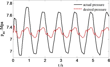
Fig. 11The sprung acceleration

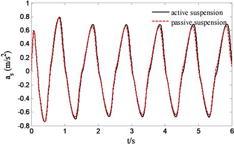
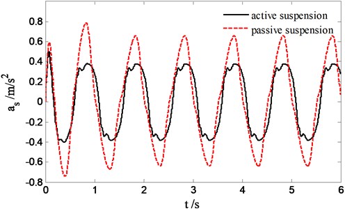
Fig. 12 suggests the force tracking effect of sliding mode controller to desired pressure $p_{d e s}$ of skyhook reference model output. Obviously sliding mode controller is superior to PID controller in accurately force tracking. Fig. 13 reflects the improvement situation of sprung acceleration compared to passive suspension, apparently a remarkable improvement of ride quality of suspension is achieved. However, based on the tracking of desired pressure $p_{d e s}$ of reference model output, the improved ride quality will never catch up with the performance acquired by tracking desired sprung velocity of reference model output.

Fig. 12Force tracking control

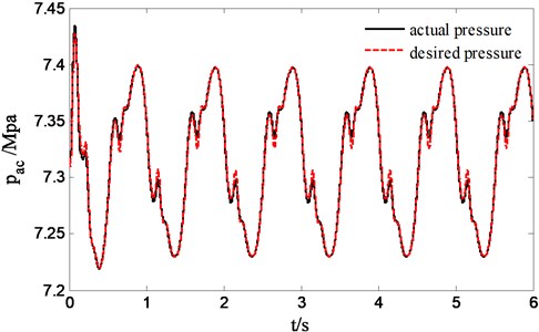
Fig. 13Sprung acceleration

7.3. Stochastic input and body control

The exciting signal of suspension is taken as standard C-class road spectrum and vehicle travel speed is set as 60 km/h. Fig. 14 reports the actual sprung velocity exactly tracks the desired sprung velocity with the proposed sliding model control algorithm for stochastic road input. Through simulation and calculation, we know that the root mean square of sprung acceleration has been improved 17.1 % over the passive suspension in the presence of 2.9 % tracking error of sprung velocity, however, the improvement only reaches to 14.05 % relative to passive suspension for the force tracking basing on desired pressure $p_{d e s}$ , and the tracking error is about 6.71 %. So the conclusion can be drawn that the suspension ride improvement based on sprung velocity tracking control is better than the effect of force tracking control based on desired force. If we can find an optimal $μ^{*}$ , apparently the tracking error of sprung velocity could be further reduced.

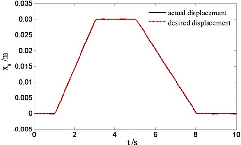
Because the sliding mode solver takes as an integral control form of tracking error of sprung velocity, which can be seen in Eq. (24), it leads to the possibility to adjust the body displacement of suspension. A step curve of sprung velocity needed to track by sliding mode solver is given in Fig. 15, which has been filtered to smooth rising edge and falling edge of step signal to prevent system oscillations in simulation. From Fig. 16, we can see that the body displacement can be controlled in a high accuracy range with the proposed double loop sliding control strategy.

Fig. 14Sprung velocity

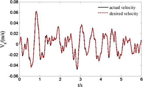
Fig. 15Step signal

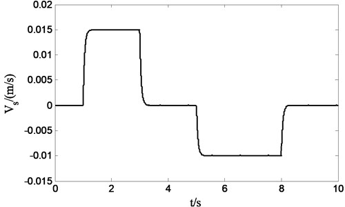
Fig. 16Body displacement

8. Conclusions

Hydro-pneumatic spring actuator is an appropriate structure way of active suspension, however active hydro-pneumatic suspension system is a complex nonlinear dynamic system coupling mechanical with electrical, hydraulic and pneumatic system each other, that give rise to challenges to realize the force tracking control for AHP system. This paper employs power bond graph theory to take carefully consideration for all aspects of the AHP system to establish the nonlinear model, and the generation and control mechanism of hydro-pneumatic spring activation force is studied based on the established model. A double-loop sliding mode control strategy and sliding mode solver stabilization control algorithm existing optimal $μ^{*}$ making sliding boundary layer smallest are presented. It realizes accurate tracking of actuation force and meanwhile reaches the purposes of the ride quality improvement of vehicle active suspension and vehicle attitude adjustment.

References

HrovatD. Survey of advanced suspension developments and related optimal control application. Automatica, Vol. 33, 1971, p. 1997-1781.

Search CrossRef
Engelman G, Rizzoni G. Including the force generation process in active suspension control formulation. Proceedings of the American Control Conference, 1993.

Search CrossRef
Alleyne A. Nonlinear and Adaptive Control with Applications to Active Suspensions. Doctoral Dissertation, UC Berkeley, 1994.

Search CrossRef
Alleyne A., Neuhus P. D., Hedrik J. K. Application of nonlinear control theory to electronically controlled suspensions. Vehicle System Dynamics, Vol. 22, 1993, p. 309-320.

Search CrossRef
Alleyne A., Liu R. On the limitations of force tracking control for hydraulic servo systems. Journal of Dynamic Systems, Measurement and Control, Vol. 121, Issue 2, 1999, p. 184-190.

Search CrossRef
Zhang Y., Alleyne A. A practical and effective approach to active suspension control. Proceedings of the 6th International Symposium on Advanced Vehicle Control, Hiroshima, Japan, September, 2002.

Search CrossRef
Lin Jung-Shan, Kanellakopoulos Ioannis Nonlinear design of active suspensions. The 34th IEEE Conference on Decision and Control, New Orleans, LA, 1995, p. 45-58.

Search CrossRef
Donahue Mark D. Implementation of an Active Suspension. Preview Controller for Improved Ride Comfort. B. S. Boston University, 1998.

Search CrossRef
Sam Y. M., Hudha K. Modeling and force tracking control of hydraulic actuator for an active suspension system. Proceeding of Industrial Electronics and Applications, 2006.

Search CrossRef
Chantranuwathana Supavut, Peng Huei Adaptive robust force control for vehicle active suspensions. International Journal of Adaptive Control and Signal Processing, Vol. 18, 2004, p. 83-102.

Search CrossRef
Chen Hong-Ming Design of a nonlinear controller for a quarter vehicle active suspension system. IEEE International Symposium on Computer, Consumer and Control, Taichung, Taiwan, 2012, p. 512-515.

Search CrossRef
Emami M. D., Mostafavi S. A., Asadollahzadeh P. Modeling and simulation of active hydro-pneumatic suspension system through bond graph. Mechanika, Vol. 17, Issue 3, 2011, p. 312-317.

Search CrossRef
Shi J.-W., Li X.-W., Zhang J.-W. Feedback linearization and sliding mode control for active hydro-pneumatic suspension of a special-purpose vehicle. Proceedings of the Institution of Mechanical Engineers, Part D: Journal of Automobile Engineering, Vol. 224, Issue 1, 2010, p. 41-53.

Search CrossRef
Akar M., Kalkkuhl J. C., Suissa A. Vertical dynamics emulation using a vehicle equipped with active suspension. Proceedings of the 2007 IEEE Intelligent Vehicles Symposium Istanbul, Turkey, 2007.

Search CrossRef
Merritt H. E. Hydraulic Control Systems. Wiley and Sons, 1967, p. 8-17.

Search CrossRef
Kroneld P. Modeling a selective hydro-pneumatic suspension element. The 13th International Congress on Sound and Vibration, Vienna, Austria, 2006.

Search CrossRef
Khalil Hassan K. Nonlinear Systems. 2nd Edition, Prentice Hall, New Jersey, 1996.

Search CrossRef
Slotine J. J. Applied Nonlinear Control. Prensey-Hall, Inc., Englewood Cliffs, New Jersey, 1992, p. 286-287.

Search CrossRef

About this article

Received

25 September 2015

Accepted

12 December 2015

Published

15 February 2016

SUBJECTS

Vibration in transportation engineering

Keywords

active hydro-pneumatic suspension

sliding mode control

force tracking

actuator

stabilization

This is an open access article distributed under the Creative Commons Attribution License, which permits unrestricted use, distribution, and reproduction in any medium, provided the original work is properly cited.