State estimation based on unscented Kalman filter for semi-active suspension systems

Lin, Cheng; Liu, Wei; Ren, Hongbin

Journal of Vibroengineering

Browse Journal

Submit article

Published: 15 February 2016

Check for updates

State estimation based on unscented Kalman filter for semi-active suspension systems

Cheng Lin¹

Wei Liu²

Hongbin Ren³

^{1, 2}Collaborative Innovation Center of Electric Vehicles in Beijing, Beijing, China

^{3, 1, 2}School of Mechanical Engineering, Beijing Institute of Technology, Beijing, China

Corresponding Author:

Wei Liu

Cite the article Download PDF

Downloads 1629

Abstract

In this paper, a novel approach to estimate vehicle vibration state information in real time is proposed; it is based on unscented Kalman filter (UKF) theory. The UKF is based on the unscented transfer technique which considers high order terms during the measurement and update stage during the estimation. The proposed observer uses easily accessible measurements such as accelerations and suspension deflections to estimate the sprung and unspring mass vertical velocity for the suspension systems of full vehicle under unknown road disturbance. And it is with low sensitivity and robust to the unknown road surfaces. Matlab/Carsim co-simulation experiments are carried out to validate the performance of the estimator under two typical road excitations. The simulation results clearly indicate that the proposed UKF sate observer is precise.

1. Introduction

State estimation is to identify the internal state information of a real system by combining information obtained from measurements of the input and output of the real system. Knowing the system state is necessary to design the controller or online fault diagnosis for a given system, such as stabilizing a system by using state feedback, PID control, et al. And the performance of the controllers relies heavily on the precision of the vehicle states. Some of the required vehicle state information is easily to be measured by the sensors, for example, vehicle body vertical acceleration; but others are difficult to detect due to the expense, complexity and the technical limitations. Reducing sensor is a potential approach to cut down the cost and improve the reliability and performance of the controller. Tims [1] studied the approaches to reduce sensors in active suspension control, he used the suspension stroke sensor to estimate sprung mass vertical velocity, but he didn’t consider the potential for phase advance or lag in the estimation of velocity, especially for the large pitch and roll motion; this will induce the signal’s time delay. Time delay is a key issue for the active suspension control.

System dynamic control heavily depends on accurate state information. And the research of vehicle’s states and parameters online estimation are attacking more and more attentions in automobile industry. One of the principal problems in semi-active suspension control is to estimate the suspension vibration states from easily accessible measurements such as accelerations. This requires observers to produce good state estimation, such as vehicle body and wheel absolute velocities, vehicle body roll and pitch rate et al. Kyongsu [2] proposed a suspension state estimation method by measuring the acceleration signals, and the stability of observer was proved. Hernandez [3] designed Romberg observer with low sensitivity to unknown road surfaces; the simulation results show that low gain Romberg observers have the best overall performance even driving on different road excitations. An online system identification to identify sprung mass and spring stiffness based on the recursive least-squares is presented in [4].

This paper studies the state estimation for strong nonlinear suspension systems. An estimation algorithm is designed based on the UKF theory to estimate the vehicle body and wheel vertical velocity as well as roll and pitch rate by the suspension stroke and vehicle body acceleration sensors. These estimated states are necessary information for the control application of suspension systems.

The organization of this paper is follows: full vehicle and the hydro-pneumatic suspension are modelling in Section 2; the state observer design and UKF theory are explained, respectively in Section 3; the effects of the proposed observer are validated by numerical simulation under two different road types in Section 4.

2. Vehicle dynamic modeling

The full-scale nonlinear vehicle model considering the heave-pitch-roll motion is necessary in development of vehicle technologies, such as suspension control, chassis integrated control, active safety, driving assistant technology, etc.

The sprung mass includes the chassis, which consists of internal components and passengers, and the sprung mass varies with the number of passengers and the payload condition of a car. It connects the suspension systems to four wheels (unsprung masses). The chassis is free to heave, pitch, and roll. The four wheels bounce vertically relatively to the vehicle body. The hydro-pneumatic suspension systems are used in this study. The damping forces can be continuously adjusted by controlling the current of the proportional relief valve according to the control algorithm. $m_{u}$ is the unsprung mass, which is supported by the tire, the stiffness coefficient of tire is $K_{t}$ . The sprung and unsprung mass displacement of are denoted as $z_{s}$ and $z_{u}$ , respectively. The road excitation is $q$ .

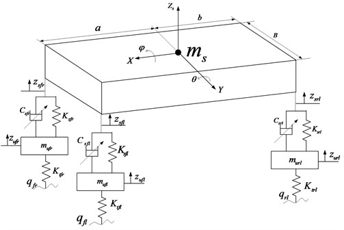
Fig. 1. Full-scale vehicle semi-active suspension model

The differential equations including vertical, pitch and roll motions are expressed as:

1

m_{s} {\ddot{z}}_{s} + \sum F_{s u s i j} = 0, i j = f l, f r, r l, r r,

2

I_{y} \ddot{θ} + a (F_{s u s f l} + F_{s u s f r}) - b (F_{s u s r l} + F_{s u s r r}) = 0,

3

I_{x} \ddot{φ} + \frac{B}{2 (F_{s u s f l} + F_{s u s r l} - F_{s u s f r} - F_{s u s r r})} = 0,

where, $F_{s u s}$ is the total suspension force including the spring force and damping force; and is generated by the hydro-pneumatic suspension. It can be described by using a nonlinear function:

4

F_{s u s i j} = F (Δ {z_{s}}_{i j}, Δ {\dot{z}}_{s i j}, u_{i j}), i j = f l, f r, r l, r r,

where, $u_{i j}$ is the control current; $f l$ , $f r$ , $r l$ , $r r$ denote front-left, front-right, rear-left, rear-right of the vehicle body.

The dynamic equations of four wheels’ vertical motion are as follows:

5

m_{u i j} {\ddot{z}}_{u i j} - F_{s u s i j} + k_{t i j} (z_{u i j} - q_{i j}), i j = f l, f r, r l, r r .

The damping continuous hydro-pneumatic suspension consists of an accumulator and a cylinder. The accumulator is filled with pre-charge gas, and it works as a nonlinear spring in hydro-pneumatic suspension system. The spring force can be calculated by:

6

F_{s i j} = \frac{m_{s} g}{4} {(1 / (1 + \frac{m_{s} g (z_{2} - z_{1})}{4 P_{0} V_{0}}))}^{r},

where, $P_{0}$ is initial pressure in the accumulator; $V_{0}$ is initial accumulator volume.

Fig. 2Suspension bench test

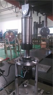
Fig. 3Spring force comparison between bench test and simulation

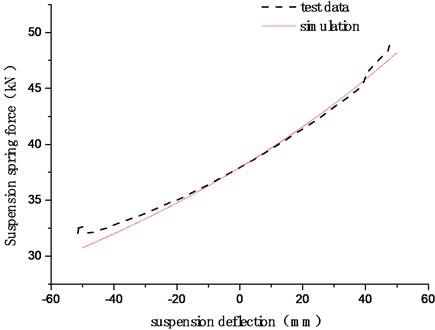
The bench test of hydro-pneumatic suspension is shown in Fig. 2. And the spring force comparison between bench test and simulation is shown in Fig. 3. The damping continuous adjustable suspension is based on the by-pass principle using a proportional relief valve in parallel with a conventional damper orifice and valve assembly. If the bypass valve is closed, all the flow goes through the conventional damper orifice and valve assembly, presenting hard-damping characteristic. If the bypass valve is open partially or totally, most of the flow will pass through the bypass valve due to the lower flow resistance, and the damping characteristic will be soft mode.

The current-velocity-damping force is fitted by a high-order polynomial function, as shown in Fig. 4. It is easy to calculate the control current to generate a desired damping force. It can be described as follows:

7

F = \sum_{i = 0}^{5} {(b_{i} I^{2} + c_{i} I + d_{i}) Δ \dot{z}}_{s}^{i},

where, $b_{i}$ , $c_{i}$ and $d_{i}$ are the fitting coefficients obtained from the experimental data. The values of these coefficients are listed in Table 1.

Table 1Coefficients of the polynomial function

$b$	Values	$c$	Values	$d$	Values
$b_{0}$	–108.67	$c_{0}$	–812.59	$d_{0}$	1035.77
$b_{1}$	–4172.29	$c_{1}$	47632.73	$d_{1}$	–2546.27
$b_{2}$	–5960.93	$c_{2}$	4939.83	$d_{2}$	–3108.31
$b_{3}$	5755.10	$c_{3}$	–79007.97	$d_{3}$	22568.64
$b_{4}$	5242.83	$c_{4}$	–5593.96	$d_{4}$	2257.40
$b_{5}$	–2448.37	$c_{5}$	44306.14	$d_{5}$	–12670.56

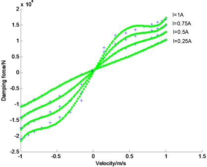
Fig. 4. Current-velocity-damping force fitting results (the dotted line is test data; the continuous line is the fitting results. When $Δ {\dot{z}}_{s} < 0$ , the suspension is in rebound motion)

The control current can be obtained according to the suspension relative velocity and the desired damping force which is determined according the control logic.

8

\sum_{i = 0}^{5} b_{i} v^{i} I^{2} + \sum_{i = 0}^{5} c_{i} v^{i} I + \sum_{i = 0}^{5} d_{i} v^{i} - F = 0 .

3. UKF observer design

In the semi-active suspension control application, some states are difficult to be measured, and some of them cannot be measured at all due to the high cost or limitations of technology. So it is necessary to design the observer to identify the states or parameters of the suspension systems, such as sprung mass vertical velocity. Kalman filtering (KF) is based on linear quadratic optimal theory, as shown in Fig. 5, which estimates unknown variables from easily measured signals. Extend Kalman filter (EKF) is a frequently used for optimal nonlinear system state and parameters estimation. EKF is based on the one-order Taylor series expansions to convert the nonlinear system into linearized one. It works well for the weakly nonlinear systems; for the strong nonlinear system, the estimation performance is not good because of high calculation cost of the system’s Jacobian matrixes. And this estimation algorithm can induce a large error in the actual values of mean and covariance, which may lead to sub-optimal performance and sometimes even cause divergence of the filter [10].

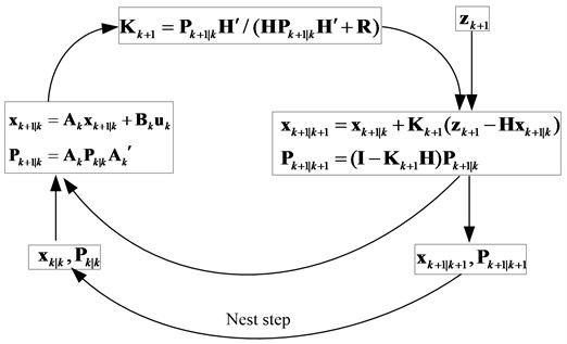
Fig. 5. Flowchart of Kalman filter

UKF is also a nonlinear Kalman filter. It is based on the Unscented Transform (UT) theory and statistical linearization technique. This technique is a new approximation method by propagating means and covariance through nonlinear transformations. The UKF is more accuracy than the EKF in terms of speed of convergence and robustness; the computational load of UKF is almost same to the EKF algorithm [10].

3.1. UT theory

The Unscented Transfer (UT) is a mathematical tool for calculating the statistics of a random variable which undergoes a nonlinear transformation, named as sigma points. The sigma points are a set of points which have mean and covariance equal to the given mean and covariance. The elements of sigma points are discrete in probability distribution. This distribution can be propagated exactly by applying the nonlinear function to each point.

In the paper, the symmetrically sampling method is used to pick up the sigma points. For the random variable state vector $x$ , the mean is $\bar{x}$ and the covariance of $x$ is denoted as $P^{x}$ . The sigma points are chosen so that their mean and covariance are exactly equal to $\bar{x}$ and $P^{x}$ respectively. Define $χ_{k}$ as a set of $2 n + 1$ sigma points [11]:

9

χ_{k} = \{\begin{array}{l} \bar{x}, & k = 0, \\ \bar{x} + (\sqrt{(n + λ) P^{x}})_{k}, & k = 1,2, \dots, n, \\ \bar{x} - (\sqrt{(n + λ) P^{x}})_{k - n}, & k = n + 1, \dots, 2 n, \end{array}

where, $n$ is the dimension of the state vector $x$ ; $λ$ is scaling parameter, $λ = α^{2} (n + κ) - n$ ; the constant $α$ is used to indicate the distribution of sigma around vector $\bar{x}$ , and the value of $α$ usually is a very small value no more than one; $κ \geq 0$ will keep the matrix of covariance to be positive definite. ${(\sqrt{(n + λ) P^{x}})}_{k}$ is the $k$ th column of the matrix square root.

3.2. UKF estimation

The sigma vectors can be renewed by:

10

χ_{k + 1} = χ_{k} + f (χ_{k}, u_{k + 1}, w_{k + 1}) \cdot Δ T,

where, $Δ T$ is system sampling time; $f$ is system function; $u_{k + 1}$ is the system input; $w_{k + 1}$ is the process Gaussian white noise with covariance $Q$ .

Measurement elements update:

11

Y_{k + 1} = h (χ_{k + 1}, u_{k + 1}, v_{k + 1}),

where, $h$ is measurement function; $v_{k}$ is the observation Gaussian white noise with covariance $R$ .

The updated state vector $x_{k + 1}$ and the measurement value $y_{k + 1}$ can be calculated by weighted sigma vectors:

12

x_{k + 1 | k} \approx \sum_{i = 1}^{2 n + 1} (W_{_{i}}^{m} {(χ_{k + 1})}_{i}), \begin{array}{l}  \end{array} y_{k + 1} \approx \sum_{i = 1}^{2 n + 1} (W_{_{i}}^{m} {(Y_{k + 1})}_{i}) .

Covariance update. The state vector and the measurement vector covariance can be renewed by:

13

P_{^{_{k + 1 | k}}}^{x} = \sum_{i = 1}^{2 n + 1} [W_{i}^{c} ((χ_{k + 1})_{i} - x_{k + 1}) ((χ_{k + 1})_{i} - x_{k + 1})'] + Q,

P_{^{_{k + 1}}}^{y} = \sum_{i = 1}^{2 n + 1} [W_{i}^{c} ((Y_{k + 1})_{i} - y_{k + 1}) ((Y_{k + 1})_{i} - y_{k + 1})'] + R,

P_{^{_{k + 1}}}^{x y} = \sum_{i = 1}^{2 n + 1} [W_{i}^{c} ((χ_{k + 1})_{i} - x_{k + 1}) ((Y_{k + 1})_{i} - y_{k + 1})'],

where:

14

W_{i}^{m} = [\frac{λ}{n + λ}, \underset{2 n}{\underset{⏟}{\frac{\frac{1}{2}}{n + λ}, \dots, \frac{\frac{1}{2}}{n + λ}}}],

W_{i}^{c} = [\frac{λ}{n + λ} + 1 - α^{2} + β, \underset{2 n}{\underset{⏟}{\frac{\frac{1}{2}}{n + λ}, \dots, \frac{\frac{1}{2}}{n + λ}}}] .

In which, $β$ considers the high order moment of the prior distribution, for Gaussian distribution, $β = 2$ is optimal.

State correction

15

K_{k + 1} = P_{k + 1}^{x y} (P_{k + 1}^{y})^{- 1},

x_{k + 1 | k + 1} = x_{k + 1 | k} + K_{k + 1} (z_{k + 1} - y_{k + 1}),

P_{k + 1 | k + 1}^{x} = P_{k + 1 | k}^{x} - K_{k + 1} P_{k + 1}^{y} (K_{k + 1})^{'},

where, $z_{k + 1}$ are the measurements from the sensors.

3.3. Suspension state estimation

Choose the state vector as $x = [\begin{array}{l} {\dot{z}}_{s} & \dot{φ} & \dot{θ} & {\dot{z}}_{u 1 ~ 4} & f_{d 1 ~ 4} & (q - z_{u})_{1 ~ 4} \end{array}]^{T}$ , and choose $h (x) = [x_{8 ~ 12}, {\ddot{z}}_{s 1 ~ 4}]^{Τ}$ , i.e. four suspension strokes and four sprung mass vertical accelerations as observer measurements. The system function can be rewritten as state-space format:

16

\{\begin{array}{l} \dot{x} = f (x) + G \cdot w, \\ y = h (x) + v, \end{array}

where, $w = \dot{q}$ is the process noise, which is the derivative of road disturbance and it is a white noise with covariance $Q$ ; $v$ is the measurement noise assumed to be zero mean Gaussian white noise with covariance $R$ .

$x_{1} = {\dot{z}}_{s}$ is vertical velocity of vehicle body mass center; $x_{2} = \dot{φ}$ is velocity body roll rate; $x_{3} = \dot{θ}$ is velocity body pitch rate; $x_{4 ~ 7} = {\dot{z}}_{u 1 ~ 4}$ is unsprung mass vertical velocities; $x_{8 ~ 11} = f_{d 1 ~ 4}$ is suspension stroke rates of four corners; $x_{12 ~ 15} = (q - z_{u})_{1 ~ 4}$ is vertical displacements of wheels.

The continuous system functions of vehicle’s dynamics function (16) could be converted as discrete-time form by using the first-order approximation, as follows:

17

\{\begin{array}{l} x_{k + 1} = x_{k} + (f (x_{k}) + G \cdot w_{k}) Δ T, \\ y_{k + 1} = h (x_{k + 1}) + v_{k + 1} . \end{array}

The state observer of nonlinear suspension system is designed; the flowchart of observer is shown in Fig. 5. Here the derivative of road disturbance is considered as system process noise. The observer is low sensitivity to unknown random road disturbances.

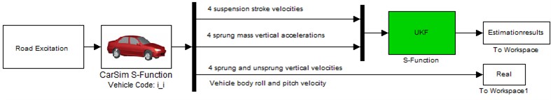
Fig. 6. The flowchart of suspension state observer

4. Simulation and discussion

In order to demonstrate the effectiveness of the proposed semi-active suspension control algorithm, it is validated in the Matlab/Simulink and Carsim co-simulation environment. CarSim is a commercial software which is widely used to simulate the dynamic behavior of vehicles. Carsim provides measurement outputs for the observer. And the control algorithm and state observer are designed in Matlab/Simulink. The estimation performance is validated under two working conditions, random road and speed bump road. The smooth random road represents consistent excitations with wide range of frequencies; the speed bump road represents the discrete events of relatively short duration and high intensity. The vehicle parameters are list in Table 2.

Table 2Parameters of off-road vehicle suspension

Description	Symbol	Value
Sprung mass	$m_{s}$	9000 kg
Unsprung mass	$m_{u}$	250 kg
The distance of body mass center to front axis	$a$	1.94 m
The distance of body mass center to rear axis	$b$	2.56 m
Tire stiffness	$k_{t}$	1501.2 kN/m
Roll moment of inertia	$I_{x}$	3531 kg∙m²
Pitch moment of inertia	$I_{y}$	16243 kg∙m²
Track width	$B$	1.481 m
Leverage ratio	$l$	1.507
Initial pressure of accumulator	$P_{0}$	8 MPa

4.1. Case 1. Random road modeling

The power spectral density (PSD) of the random road model can be described as the following form:

18

G_{q} (n) = G_{q} (n_{0}) {(n / n_{0})}^{- w},

where, the space frequency is denoted as $n$ (m^-1); $n_{0}$ is the reference space frequency, $n_{0} =$ 0.01 m^-1; $G_{q} (n_{0})$ is the road roughness coefficient, here, choose $G_{q} (n_{0}) = 256×1 0^{-6}$ ; $w$ is frequency index, it reflects the frequency structure of the road model, usually $w = 2$ .

The random road excitation model can be acquired by integration of Gaussian white noise. The random road differential equation can be described as [12]:

19

\dot{q} (t) = 2 π n_{0} \sqrt{G_{q} (n_{0}) u} W (t) - 2 π n_{00} u q (t),

where, $W (t)$ is the Gaussian white noise; $n_{00}$ is the low cut-off space frequency, $n_{00} = 0.001 m^{-1}$ ; $u$ is the vehicle longitudinal speed.

The four wheels road excitation can be referenced to the method proposed by Ren et al. [13]. The vehicle speed is kept constant as 60 km/h, and the four wheels of irregular road profiles are plotted in Fig. 7. The estimation results are presented in Figs. 8-12. Fig. 9 is the vehicle body mass center vertical velocity estimation results. Fig. 9 and Fig. 10 plot the vehicle body roll and pitch rate estimation results. Fig. 11 and Fig. 12 are the vehicle body and wheel vertical velocity estimation results. From the estimation results, we can find that compared with the EKF estimation results, the UKF state observer could estimate the suspension state in accurate when vehicle is driving on the random road.

4.2. Case 2: speed bump road

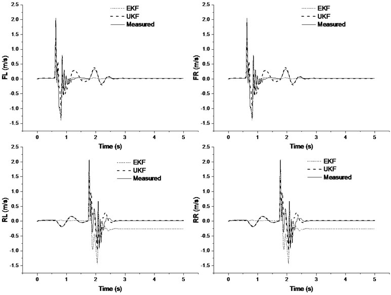
The speed bump road can certainly do harm if drive over them too quickly, and it cause large motion of vehicle body in a short time. In the numerical simulation, the vehicle velocity is kept constant as 30km/h. Time history of speed bump road is plotted in Fig. 13. The estimation results are presented in Figs. 14-17. It can be found that the UKF observer could estimate the suspension states in precise when vehicle is crossing the speed bump road.

Fig. 7Time history of four wheels disturbance input

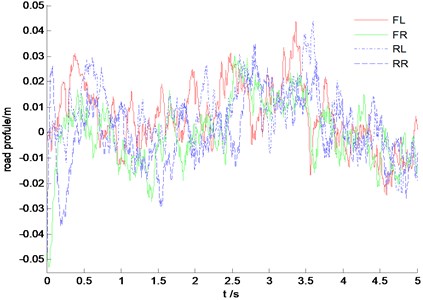
Fig. 8Vehicle body mass center vertical velocity estimation results

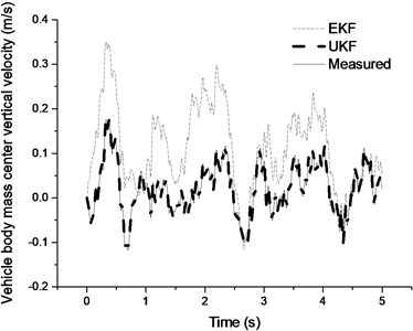
Fig. 9Roll velocity estimation results

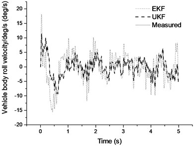
Fig. 10Pitch velocity estimation results

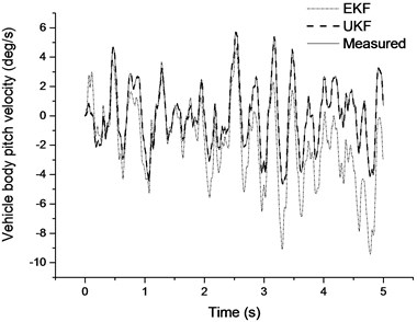
Fig. 11Sprung mass vertical velocity estimation results

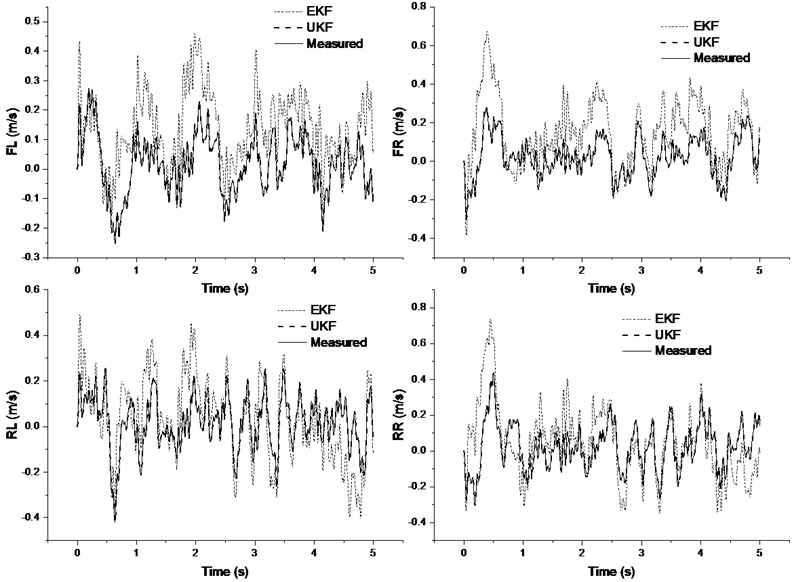
Fig. 12Unsprung mass vertical velocity estimation results

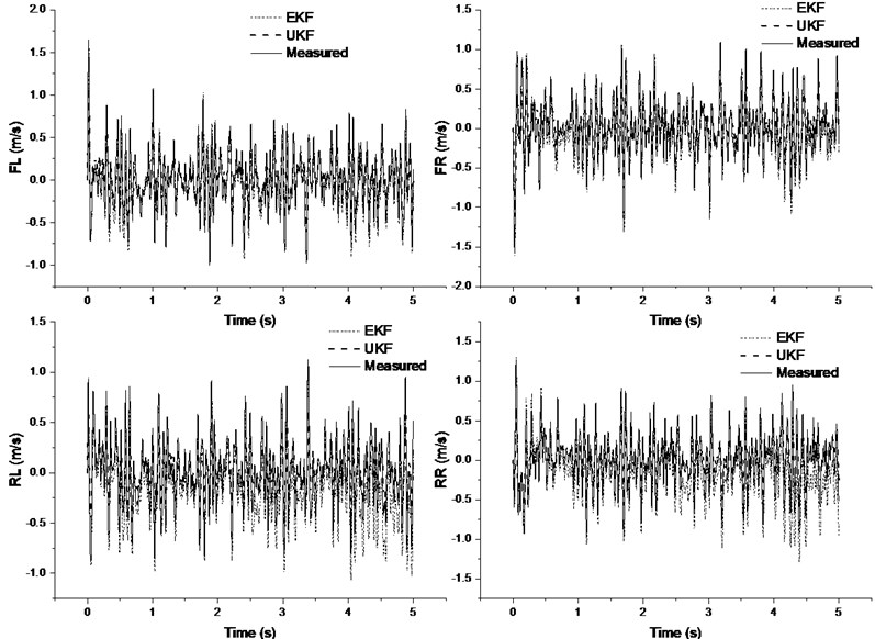
Fig. 13Time history of speed bump road input

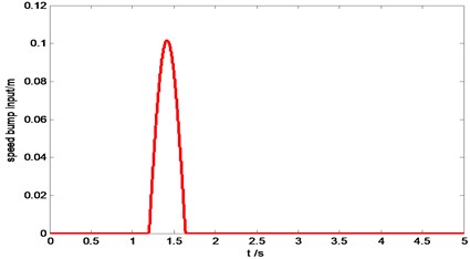
Fig. 14Vehicle body mass center vertical velocity estimation results

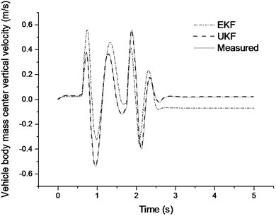
Fig. 15Pitch angle velocity estimation results

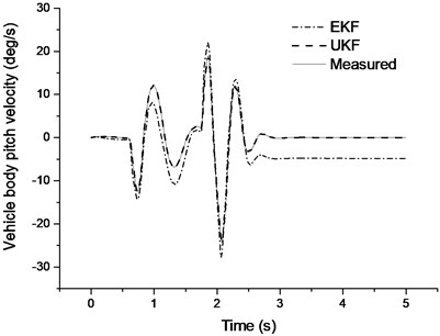
Fig. 16Sprung mass vertical velocity estimation results

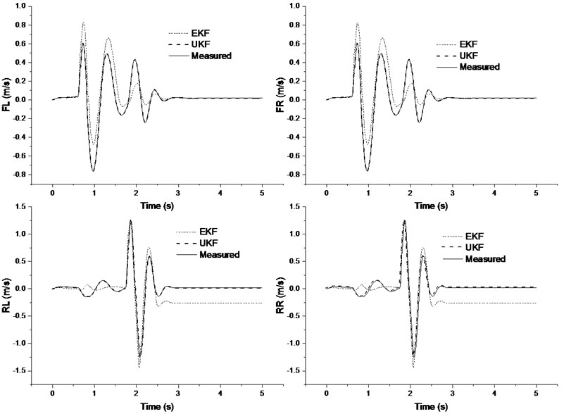
Fig. 17Unsprung mass vertical velocity estimation results

5. Conclusion and future work

The suspension state observer with low sensitivity to road disturbance is designed based on UKF theory for nonlinear suspension systems. The UKF observer is successfully in estimating the state information of the suspension vibration with good accuracy. The performance of the proposed estimator is validated on two typical road excitations. The simulation results indicated that compared with the EKF estimation results, the performance of the designed UKF observer is more precise. The future work should be concentrating on validating the designed observer algorithms in the vehicle tests.

References

Tims H. Vehicle Active Suspension System Sensor Reduction. Ph.D. Thesis, University of Texas, Austin, Tex, USA, 2005.

Search CrossRef
Yi Kyongsu, Song Byung Suk Observer design for semi-active suspension control. Vehicle System Dynamics, Vol. 32, Issues 2-3, 1999, p. 129-148.

Search CrossRef
Hernandez-Alcantara Diana, Amezquita-Brooks Luis, Morales-Menendez Ruben State-Observers for Semi-Active Suspension Control Applications with Low Sensitivity to Unknown Road Surfaces. SAE Technical Paper No. 2014-01-0867, 2014.

Search CrossRef
Best, M. C., Gordon T. J. Suspension system identification based on impulse-momentum equations. Vehicle System Dynamics, Vol. 29, Issue 1, 1998, p. 598-618.

Search CrossRef
Zong C., Hu D., Zheng H. Dual extended Kalman filter for combined estimation of vehicle state and road friction. Chinese Journal of Mechanical Engineering, Vol. 26, Issue 2, 2013, p. 313-324.

Search CrossRef
Ren H., Chen S., Shim T., Wu Z. Effective assessment of tyre-road friction coefficient using a hybrid estimator. Vehicle System Dynamics, Vol. 52, Issue 8, 2014, p. 1047-1065.

Search CrossRef
Ren H., Chen S., Liu G., et al. Vehicle state information estimation with the unscented Kalman filter. Advances in Mechanical Engineering, 2014, p. 1-11.

Search CrossRef
Lu Fan Study on Vehicle Vibration State Observation Algorithm Based on the Nonlinearity of Suspension. Ph.D. Thesis, Beijing Institute of Technology, Beijing, China, 2014.

Search CrossRef
Beltran Carbajal Francisco, et al. Active disturbance rejection control of a magnetic suspension system. Asian Journal of Control, Vol. 17, Issue 3, 2015, p. 842-854.

Search CrossRef
Wan Eric, van der Merwe Rudolph Kalman Filtering and Neural Networks. Chapter 7: The Unscented Kalman Filter. Wiley Publishing, 2001.

Search CrossRef
Rambabu Kandepu, Foss Bjarne, Imsland Lars Applying the unscented Kalman filter for nonlinear state estimation. Journal of Process Control, Vol. 18, Issue 7, 2008, p. 753-768.

Search CrossRef
Wu Z., Chen S., Yang L., et al. Model of road roughness in time domain based on rational function. Transactions of Beijing Institute of Technology, Vol. 29, Issue 9, 2009, p. 795-798.

Search CrossRef
Hongbin R., Sizhong C., Zhicheng W. Model of excitation of random road profile in time domain for a vehicle with four wheels. The Proceedings of the International Conference on Mechatronic Science, Electric Engineering and Computer, Jilin, China, 2011, p. 2332-2335.

Search CrossRef

About this article

Received

02 September 2015

Accepted

13 December 2015

Published

15 February 2016

SUBJECTS

Vibration in transportation engineering

Keywords

nonlinear suspension system

UKF

state estimation

co-simulation

Acknowledgements

The authors acknowledge that this paper has been supported by National Natural Science Foundation of China (No. 51575044).

This is an open access article distributed under the Creative Commons Attribution License, which permits unrestricted use, distribution, and reproduction in any medium, provided the original work is properly cited.