Abstract
Considering easy determination of natural frequency in structures leads researchers to focus on detecting the damage through the dynamic parameters using combination of various artificial intelligence algorithms. The main contribution of this research is to detect damage in structures (including its depth and location) for the deep beams with Timoshenko behavior using optimization via simulation (OVS). This method is established based on the first three natural frequencies of the deep or semi-deep beams. The finite element method (FEM) is conducted to obtain essential inputs parameters for OVS. The exact location and depth of the structural damage are determined, using combination of multi-objective optimization algorithms, multi-objective genetic algorithm (MOGA), and modified multi-objective genetic algorithm (MMOGA). This research also remarkably concerns about detecting the location of the defect in the beams with several cracks. In order to verify the results obtained from numerical analysis, several experimental specimens are presented. The dynamics parameters of the beams are experimentally identified using modal hammer. The responses obtained from the numerical method, proposed in this research, are also compared with the results obtained from previous studies. Practically, a beam with real dimensions is examined for different boundary conditions. In addition, the results obtained from MOGA and MMOGA are compared with the other researchers’ achievements. Finally, it was observed that the proposed method, (OVS), can be satisfyingly determined the exact location and depth of damage with the high accuracy.
1. Introduction
Detecting the exact location of damage in the structures has always drawn the attention of researchers concerning the stability and deterioration of the structures. It has been pointed out as a major problem in various structures such as bridges, high-rise and mid-rise structures, concrete dams, and buildings. The structures may experience defects in their life-time due to construction ignorance, corrosion, fatigue, seismic effect, and so on. Accordingly, several methods have been developed for damage detection. These methods are mostly not applicable in reality due to the difficulties in the determination of preliminary parameters or high error levels. The previous methods have been developed based on the determination of structural properties with consideration static and dynamic responses. Static response-based methods determine deformations, stiffness, and capacity of the structural members by measuring their strain and displacement subjected to the static loads using updated Finite Element (FE) model. Kourehli et al. [1] studied incomplete static response and its combination with dynamic response. They considered dynamic methods based on the signal and modal processing information. However, the methods utilized natural frequency of preliminary modes to detect the exact location of damages.
Goldfeld et al. [2] investigated damage detection methods using modal frequency variations in the beams. They studied the distribution, intensity, and location of damages, considering the stiffness distributed in the beams and the changes appeared in the modal frequencies of any modal shapes. Accordingly, they investigated continuous cracks and their exact locations in the concrete beams. Perera et al. [3] assessed structural damage with different dimensions and certain number of elements. They identified the level and location of damages through updating dynamic and static measurements of the beams. In 2012, Seyedpoor [4] used a two-step method to detect damages based on modal strain energy index and particle optimization algorithm. He determined the level of damage using Particle Swarm Optimization (PSO) method and its exact location using modal strain energy method. In this regard, five preliminary vibration modes were used to specify the damage level. Then, the strain energy values of 15 various elements were calculated for the damaged and undamaged statuses. Miguel et al. [5] proposed a compound method for detecting the damage of structures caused by applied loads. The research was carried out in two steps: 1) discussing the experimental studies; 2) analyzing the obtained results by Genetic Algorithm (GA), Harmony Search Algorithm (HS), and Particle Swarm Optimization (PSO) methods. They used this method to determine the damage levels in noises in the 2-D portal frames and beams, regarding different noises. Miguel et al. [6] studied damage detection in the ambient vibrations mode through Harmony Search (HS) model, provided a compound method using modal technique in time domain to obtain final response of the considered structures. They presented different examples for various noises with several damages. In 2013, Esfandiari et al. [7] studied the damage numerically and experimentally using natural frequency based on modified sensitivity equations. This technique specifies the structural damage based on the frequency and stiffness reduction level. They evaluated the behavior of structure under the damage effects considering modal shape, frequency and solving the equations in each mode. In 2013, Mehrjoo et al. [8] investigated Genetic Algorithm (GA) and its application in damage detection of beam-shape components with Bernoulli beam elements. They considered the crack using rotational mass-less spring in 2-D and 4-node elements. Accordingly, the crack stiffness was introduced as (rotational spring stiffness) in the numerical solution method. They specified the location, depth and damage level of the crack using natural frequency. Su et al. [9] attempted to detect the damage in the stories of a 2-D portal frame using its natural frequencies. They applied optimization algorithm such as Genetic Algorithm in their research. Obviously, any changes in the mass properties and stiffness of beams results in the determination of damage intensity. This discussion can be generalized to 2-D structures with shear behavior such that the behavior of structure changes in the floor with stiffness reduction or mechanical properties. The amount of the damage can be detected by investigating its corresponding frequencies. According to this hypothesis, the stiffness of damaged floor is a percentage of other floors’ stiffness. Moreover, the acceleration response is considered independently in each floor. Baghmisheh et al. [10] proposed a new optimization method to detect damage in a cantilever beam. They compared different optimization methods such as GA, PSO, and etc. in their research. Zheng et al. [11] assessed modal frequencies for the beams layered by glass and epoxy in different sizes at different locations using Radial Fuzzy Genetic Algorithm (RBF). They measured structural properties such as frequencies using FEM and identified damage location. Moreover, they applied Genetic Algorithm in order to solve and control the problem. Meruane et al. [12] used integrated Genetic Algorithm for identifying the structural damage and modal properties in order to obtain the exact location of damage and its intensity. They considered two numerical and experimental statuses for damaged and undamaged structures to investigate the effect of noises and computational errors.
Natural frequencies in three preliminary modes are the measurable dynamic parameters in the beam like structures. They are calculated by experimental methods such as Modal Hammer test [13], determination of ultrasonic waves in the material [14] and other similar methods. The experimental specimens are designed and tested according to American Society for Testing and Materials (ASTM) [13]. In this research the exact location and depth of crack is detected using dynamic response of the defected deep beam in the natural frequency domain and combination of that with multi-objective Metaheuristic artificial intelligence methods. In doing so, the first three natural frequencies are considered to detect the exact location of damage by new optimization method, which is developed by OVS modeling. Accordingly, steel and aluminum specimens with certain dimensions are assessed in undamaged and damaged scenarios. Based on the experimental scenarios, the efficiency of OVS method is evaluated with comparison by Ruotolo and Surace [15] and Yoon et al. [16]. In the last scenario, a big semi-deep beam with different support statuses-cantilever, clamped-clamped, simple-clamped, and simply-supported beams is analyzed to comprehensively assess the efficiency of the proposed method. Then, the location and depth of damage are detected using MOGA and MMOGA optimization algorithms.
2. Modeling
2.1. Optimization via simulation (OVS)
OVS is an expanding method with respect to its existence complexity in the engineering issues. The model has been used very often in different engineering fields [17]. The method is generally applied to solve the issue for continuous or discrete problem. OVS is defined according to [17] as follows:
where, is a single or multi-dimensional variable, herein a 2-D variable including the defect depth and its distance from support; and is a parameter indicating the activity domain. does not have a precise solution method (closed-form) is a variable in optimization system; and is the function of optimization output. Generally, the objective function of OVS is to find minimum, maximum or target values for . and are depth and distance of defect from support, respectively; and are the first three natural frequencies of structure. Fig. 1 presents general framework of OVS method.
In order to solve a problem by OVS, first, some populations are taken from continuous model and classified as discrete input in the form of Metaheuristic algorithms. In this research, MOGA and MMOGA are considered.
Fig. 1OVS based on [17]
![OVS based on [17]](https://static-01.extrica.com/articles/16681/16681-img1.jpg)
2.2. MOGA and MMOGA
Final response-based multi-objective optimization methods are required to consider several limitations and conditions. MOGA is one of the best and oldest optimization methods. Fig. 2 depicts MOGA based on the modified population out of preliminary parents.
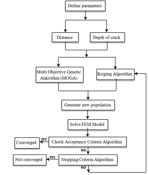
One important part of optimization algorithms is how to made and generate the populations in each analysis and repetition stage. Various methods can be applied to generate basic population such as Monte Carlo [18], Latin Hypercube Sampling [19], and Space-Filling Model [20]. These methods include each their own applications for different engineering issues. In MOGA, the populations are randomly generated, however, in MMOGA the populations are generated based on Kriging algorithm. Concerning MMOGA algorithm, the output responses are improved, adjusted with higher level variables, and presented in two-dimensional forms. Kriging algorithm [21-24] is a precise multi-dimensional interpolation using a simple polynomial function. Its efficiency can be maximized based on the capability of estimating the errors and modifying the preliminary population. Crossover and mutation are two parameters effective in the two mentioned optimization methods. The latter indicates the inheritance from parents. In the other words, some information of parents is transmitted to children, a value between zero and one. The closer the value is to zero, the more the children are similar to parents. The closer the value is to one, the more different the next generation is from its parents. In this research, this value is set as 0.98, close to one, to maximize the accuracy of calculations. The former describes the changes in the value of one or more genes in one chromosome relative to the preliminary status. The values are also between zero and one like those of crossover parameter. High value shows random algorithm and low value indicates the modeling of most chromosomes from previous condition. In this research, the lowest value is considered (0.01) in order to obtain more convergence and also more similarity between previous and next generations. 100 data are generated in each cycle for two methods based on trial and error.
Fig. 2Multi Objective Genetic Algorithm (MOGA)
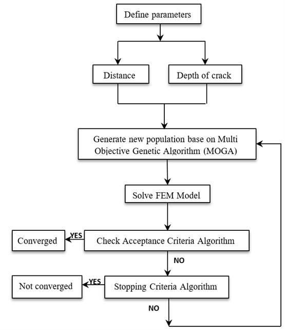
Fig. 3 shows the solving process of MMOGA. This algorithm is a Genetic Algorithm concerning its application excluding the generation and distribution of population.
Maximum allowable Pareto percentage is an acceptance criterion indicating the ratio of appropriate points to the number of samples in each iteration. The value of this parameter is considered close to one for better convergence of optimization analyses. Convergence stability percentage is a criterion for optimizing the population generated in each generation. The value of this criterion is calculated according to mean value and standard deviation. The analysis is converted and stopped when the responses obtained from optimization process are equal to the ones gained in the previous generations of optimization process. It means that the responses obtained from two subsequent generations have mean value and standard deviation of zero. The standard deviation and mean value of data are calculated based on the generated population. The standard deviation value is controlled according to Eqs. (3) and (4). If this value is equal to the previous one, the convergence has taken place. As long as these equations are not satisfied, the optimization process goes on. In these equations, the stability percentage is the distinction between two generations. If the difference between the results is lower than %, the analysis is convergent, otherwise, it continues until meeting convergence. In this analysis, the convergence value is considered as 2 %:
where, is mean value of the population in the th stage; is standard deviation in the thstage; is maximum output calculated in the preliminary generated data; and is minimum output calculated in the preliminary generated population.
Fig. 3Modified Multi Objective Genetic Algorithm (MMOGA)
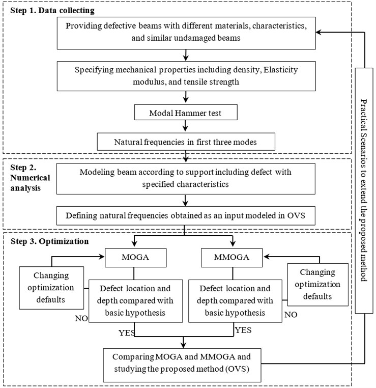
In the final stage, behavioral models are provided for two considered optimization algorithms and combined with OVS method. Then, the main problem is solved based on FEM concept. Fig. 4 presents different stages of OVS used for detecting the damages and their locations in the structures. Fig. 4 is categorized into three steps including; step 1 data collecting, step 2 numerical analysis (FEM), and step 3 optimization. In step 1 dynamic properties of the damages beam, in and its physical properties of the specimen such as density and modulus of elasticity (E) are identified using Modal Hammer test. Numerical analysis is performed based on Finite Element Method. Eventually in step 3, the obtained results are utilized as the input for optimization analysis. The location and depth of defect is identified using FEM.
The frequencies of damaged beam are calculated considering a hypothetical location for the defect. Then, the damage state is investigated for the structures comparing the frequencies of the damaged and undamaged beams based on the proposed method (OVS).
Fig. 4Modeling process of OVS for calculating actual depth and location of the damages
3. Calculating natural frequencies for Timoshenko beam
For applying optimization methods and obtaining final responses through numerical the methods, it is necessary to create the matrices of mass, stiffness and displacement vectors and investigate the structures in the damaged and undamaged conditions. In general, the transformation equations governing the vibrations of a deep beam, and its corresponding slope for undamaged Timoshenko beam, , are specified according to [25] using Eqs. (5) and (6). Besides, the strain energy is calculated according to [26] Eq. (7) as follows:
where, is material shear modulus; is shearing coefficient of deep beam with Timoshenko behavior (6/5 for rectangular profile, 10/9 for circle and 1 for I-shape profile); is material elastic modulus; is deep beam inertia; is time; and is material mass density:
where, is shape function; is slope function; is bending slope; is the first bending slope derivative; is hypothesized elements length (two node- elements with 4 degrees of freedom); and denote the mass and stiffness matrices for a deep beam with Timoshenko behavior in undamaged condition, which can be taken from Petyt. [27].
, and their derivatives can be written in form of nodal displacements to obtain equation 8 and placing support conditions, its equation is attained.
4. Experiment setup and procedure to verify proposed method
Several specimens with the characteristics mentioned in Table 1 are prepared and experimented in order to execute different research stages and verify the obtained results. Figs. 5(a) and 5(b) displays the specimens made of steel and aluminum in two damaged and undamaged conditions. For constructing cracked specimens, WIRECUT and WATERJET technologies are applied to create the thickness less than one millimeter.
Fig. 5Specimens made of steel and aluminum
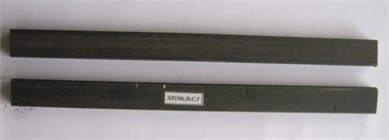
a) Creating crack in the aluminum specimens
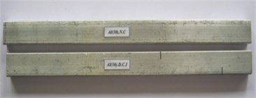
b) Creating crack in the steel specimens
For more evaluation, the damaged and undamaged specimens are compared with each other. In order to generalize the obtained results, aluminum and steel specimens are used with the material mass density of 3270 kg/m3 and 8650 kg/m3, respectively, elastic modulus of 63 GPa and 180 GPa, respectively and Poisson ratios of 0.29 and 0.35, respectively.
Two specimens, steel and aluminum, are considered undamaged (control). Besides, two other corresponding ones are constructed with the same dimensions and mechanical properties having two opposite transverse cracks of 10 mm depth (Fig. 6). The specimens have cross sections with 15 mm width, 30 mm depth, and 290 mm length. Table 1 shows the exact dimensions of specimens and the location, depth and number of their cracks.
Fig. 6The location and depth of crack in the cantilever beam of steel and aluminum specimens
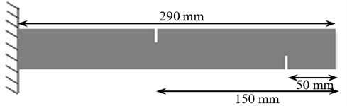
Table 1The characteristics of specimens in steel and aluminum cantilever beam
Length (mm) | Cross section (mm2) | Type | Row | Depth of crack (mm) | Distance (mm) | Crack position | Crack number | ||
No. 2 | No. 1 | No. 2 | No. 1 | ||||||
1 | ST(30).N.C | 30×15 | 290 | – | – | – | – | – | – |
2 | ST(30).D.C.I | 30×15 | 290 | 10 | 10 | 50 | 150 | 2 | Inverse |
3 | Al(30).N.C | 30×15 | 270 | – | – | – | – | – | – |
4 | Al(30).D.C.I | 30×15 | 270 | 10 | 10 | 50 | 150 | 2 | Inverse |
Fig. 7The characteristics of specimens in an aluminum cantilever beam and a steel cantilever beam, also acceleration sensor
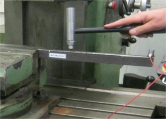
a) Aluminum cantilever beam
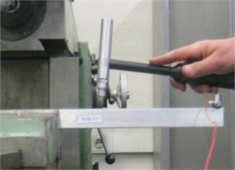
b) Steel cantilever beam
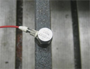
c) Acceleration sensor, (accelerometer: model-AP2037-3010)
In this research, dynamic analysis device was utilized including APTECH Company Hammer (type AU02); acceleration sensor, (accelerometer: model-AP2037-3010); data-logger (B&K); processor (PULSE analyzer platform) to measure the beam response. Fig. 7(a), (b) present an example of Modal Hammer test for cantilever beam of aluminum and steel specimens respectively. Fig. 7(c) shows the acceleration sensor with frequency range between 0.50 to 15000 Hz. During the process, which was performed using PULSE analyzer platform, the more carefully the fixed end support is created, the lower the error and noise are formed in the obtained natural frequencies. Accordingly, the weight ratio of 1000 to 1 has been considered for the supports in all specimens in order to omit noises from support mobility.
Regarding the stability and accuracy, tests are repeated several times to obtain the output stability in such a way that noises have the least effect on the results. Table 2 presents the obtained results from the tests and those of numerical modeling according to the FEM, the second column.
As an example Fig. 8 illustrates the frequency function for damaged steel specimen, which its peaks identify the first three frequencies. The obtained first three frequencies were used as the inputs for the proposed method in Fig. 4.
High accuracies of the results are confirmed by comparing the values obtained from experimental and numerical tests. Accordingly, the maximum differences between the results in the first frequency are 1 % and 2 % for the steel and aluminum specimens, respectively. In the second frequency, maximum error levels 2 % and 2.55 % in the steel and aluminum specimens, respectively, and in the third frequency 5 % and 1 %, respectively. The errors seem to be resulted from environmental noises and measuring during the tests. In the following, OVS is discussed in different samples, considering the obtained precise results.
Fig. 8Frequency response function for damaged aluminum specimen AL(30).N.C.I
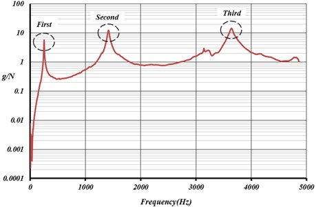
Table 2Dynamic properties of steel and aluminum cantilever beams using experimental and numerical methods
Material | Natural frequency (Hz) | ||||||
Experimental method | Numerical method (FEM) | ||||||
1st mode | 2nd mode | 3rd mode | 1st mode | 2nd mode | 3rd mode | ||
Steel | Damaged | 259.4 | 1540.0 | 3940.50 | 260.0 | 260.0 | 3945 |
Undamaged | 254.5 | 1453 | 3963 | 255.64 | 255.64 | 3777.7 | |
Aluninum | Damaged | 253.5 | 1509 | 3819.5 | 258.35 | 258.35 | 3842.8 |
Undamaged | 250.50 | 1411.52 | 3664.4 | 251.59 | 251.59 | 3673.4 | |
4.1. OVS responses using the setup experimental
In this section, the efficiency of OVS is studied regarding the obtained results from numerical and experimental tests. Fig. 6 presents the specimen configuration with cross section of 15 mm×30 mm and the length of 290 mm having cantilever support and cracks. This sample is modeled and analyzed with FEM to investigate the location and depth of its cracks through OVS as well as MOGA and MMOGA optimization methods.
In this method, the preliminary natural frequencies are considered as input for a beam with two cracks. After optimization by the above mentioned methods, two parameters, depth of the cracks and distance from the support, are obtained as the output. Accordingly, experimental results (Table 2) are used as the input parameters for optimization of MOGA and MMOGA methods.
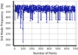
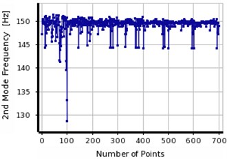
Figs. 9 and 10 present analysis results approaching towards considered responses based on MOGA and MMOGA. According to these figures, the responses are far from the target values in the first stages. Then, they show convergence in the analysis after several trial and error efforts. In the other words, the target function of optimization algorithm was satisfied when all three frequencies, simultaneously converge toward the values defined at the beginning of analysis, the test results. It is not possible to obtain precise preliminary response simultaneously. However, repeating the analysis in different data sets results in approaching the optimization values toward preliminary responses. Applying the natural frequencies, obtained from experimental results, as the input parameters, the noises also enter the optimization calculations. Concerning these inputs give us an opportunity to directly consider the noise frequency. Since filtering of the noise causes to ignore some portions of the frequency content of the response, in this research, the input data were associated with noise to demonstrate the more rational response behavior.
Fig. 9The convergence in the first three frequencies of steel cantilever beam using MOGA
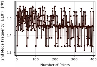
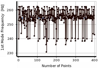
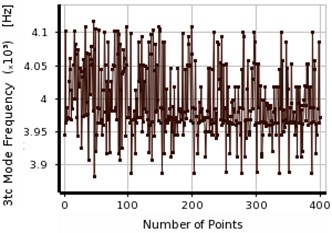
Fig. 10The convergence in the first three frequencies of steel cantilever beam using MMOGA
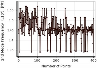
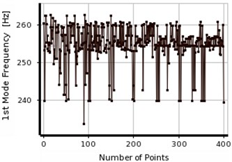
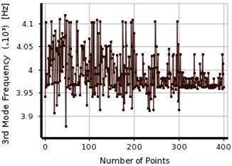
Table 3 presents the convergence of the obtained results from two considered methods, MOGA and MMOGA, for steel beam. Accordingly, three final responses of frequencies were obtained. The results related to the location and depth of the cracks shows in Table 3. The error levels are similar in both optimization methods. Three final responses were evaluated for both methods. The observations showed that error level was relatively higher in the first column of responses (Table 3), comparing to those of the second and third ones. Concerning the complementary process of optimum response selection (shown by *) the locations of the cracks were 53.59 mm and 146.82 mm in MOGA, and 54.01 mm and 158.23 mm in MMOGA, respectively. However, these values, obtained from excremental tests, were 50 and 150 mm, respectively. Using both method (MOGA and MMOGA), the depth of the crack was measured about 9 mm, which was 10 mm in reality.
Table 3The obtained results from OVS before the last step of analysis for steel cantilever beam
Method | Crack position 1 (mm) | Crack position 2 (mm) | Natural frequency (Hz) | |||||||||
Distance | Depth | Distance | Depth | 1st mode | 2nd mode | 3rd mode | ||||||
OVS | E % | OVS | E % | OVS | E % | OVS | E % | |||||
MOGA | 1 | 67.59 | 26 | 9.09 | 10 | 160.30 | 6.4 | 9.10 | 10 | 255.61 | 1449.36 | 3960.11 |
2* | 53.59 | 6.6 | 9.09 | 10 | 146.82 | 2.1 | 8.93 | 11 | 257.78 | 1455.14 | 3961.64 | |
3 | 57.98 | 13.7 | 9.20 | 8 | 169.22 | 11.3 | 8.98 | 11 | 254.01 | 1467.29 | 3979.37 | |
MMOGA | 1 | 72.87 | 31 | 9.04 | 10 | 173.28 | 13.4 | 9.65 | 3.5 | 253.36 | 1454.88 | 3966.03 |
2* | 54.01 | 7.4 | 9.67 | 3.3 | 158.23 | 5.2 | 9.22 | 7.8 | 255.64 | 1445.97 | 3965.63 | |
3 | 57.62 | 13.2 | 9.09 | 10 | 152.80 | 1.8 | 8.92 | 11 | 257.01 | 1455.88 | 3962.92 | |
Fig. 11The convergence in first three frequencies of aluminum cantilever beam using MOGA
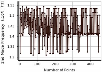

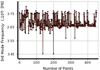
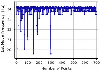
Figs. 11 and 12 show the process of obtaining the final response for aluminum beam using two considered optimization methods (MOGA, MMOGA). In Figs. 9-12, the response tolerance shows lower changes in the first frequency relative to the primary defined value in both aluminum and steel specimens, comparing to those of the second and third frequencies. In the other words, the second and third frequencies show more effects on the final response determination. In all cases, the second response shows great changes comparing to others due to its convergence in different points.
The process illustrates in Fig. 12 for three natural frequencies of aluminum specimen. MMOGA does not show sufficient accuracy in the aluminum specimens. Large variation is observed in the first and second frequencies in meeting the final response. Optimal responses do not have sufficient accuracies due to the lack of convergence in reaching the final response. Implementing the natural frequencies obtained from experimental results as input parameters, the noises existed in the information enters the optimization calculations as well. Regarding the calculations related to the defective location of aluminum beam, the noise values are 1.8 %, 2.14 % and 1 % in the first, second and third frequencies, respectively.
Fig. 12The convergence in the first three frequencies of aluminum cantilever beam using MMOGA
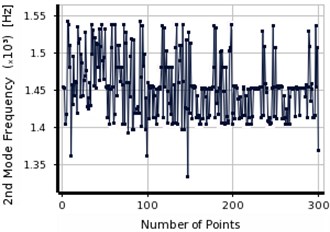
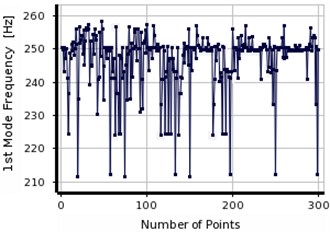
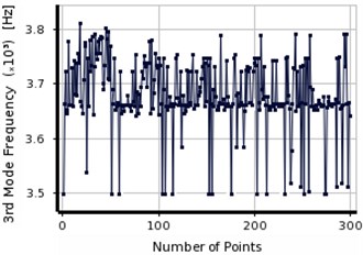
Table 4The obtained results from OVS before the last step of analysis in aluminum cantilever beam
Method | Crack position 1 (mm) | Crack position 2 (mm) | Natural frequency (Hz) | |||||||||
Distance | Depth | Distance | Depth | 1st mode | 2nd mode | 3rd mode | ||||||
OVS | E % | OVS | E % | OVS | E % | OVS | E % | |||||
MOGA | 1 | 122.74 | – | 8.59 | – | 172.0 | – | 7.40 | – | 250.68 | 1414.71 | 3659.17 |
2 | 126.7 | – | 9.42 | – | 166.03 | – | 6.74 | – | 248.62 | 1411.56 | 3658.21 | |
3* | 44.80 | 10.4 | 9.27 | 7.3 | 168.75 | 11.1 | 9.04 | 9.6 | 249.90 | 1452.15 | 3658.39 | |
MMOGA | 1 | 122.5 | – | 8.34 | – | 168.8 | – | 7.34 | – | 251.20 | 1415.64 | 3675.65 |
2 | 137.2 | – | 6.59 | – | 200.8 | – | 9.43 | – | 247.39 | 1425.37 | 3658.22 | |
3 | 173.91 | – | 8.6 | – | 151.61 | – | 7.74 | – | 247.08 | 1412.87 | 3690.74 | |
Table 4 presents the results from the final stage corresponding to the aluminum beam in three responses using two considered optimization methods. In MOGA, three obtained results are not as much similar. However, in the aluminum beam with intended conditions, the responses of the last stage are closed due to the flexibility-sensitivity of its modulus of elasticity (E). Slight variation can be observed in the frequencies with changing the location and depth of cracks causing the insufficient accuracies in the optimization responses. The responses in the third row of Table 4, (shown by *), indicate maximum accuracy of the proposed method for aluminum specimen. In MMOGA for aluminum beam, the final responses of optimization are much far from the actual value. Generally, with consideration OVS for aluminum specimens, MOGA can be recommended as the appropriate methods due to the frequencies closeness resulting from the elements flexibility. However, in the steel specimens, the results from both methods are convergent to the final response even in the pre-final stage. They easily converge to final response as the analysis goes on.
5. Experimental scenarios
5.1. Specimen No. 1
The efficiency of the proposed method was assessed through the experimental specimen with the characteristics of Fig. 13 considering the beams with two parallel cracks in line. The obtained results were verified using Ref. [15]. Accordingly, the beam is made of a material with the following properties: the Poisson’s ratio 0.29, the modulus of elasticity 180 GPa and the material mass density 7860 kg/m3. The length of specimen is 800 mm and its rectangular cross-section has 20 mm depth and 20 mm height. The cracks were formed transversally in the experimental specimen according to Fig. 13. They have the depths of 4 mm and 6 mm and the distances of 255 mm and 545 mm, respectively.
Fig. 13The location and depth of crack in cantilever beam according to [15]
![The location and depth of crack in cantilever beam according to [15]](https://static-01.extrica.com/articles/16681/16681-img24.jpg)
Table 5 presents the experimental and numerical results based on the mentioned cross section and materials properties, which were shown in Fig. 13. The error level was lower than 1 % for three frequencies, comparing the numerical and experimental results. All results show high accuracy of the modeling in the numerical method (FEM).
Table 5 shows the obtained results from experimental study, numerical method, and existing technique based on Ref. [8]. Responses closeness obtained from all three considered methods (Table 5) indicates compatibility of the outcomes of this study with conventional methods. The experimental data was considered as input for OVS based on the results given in Table 5. Two experimental and numerical cases were taken from noises tested considering different measurement errors. In the other words, the error caused by the noise was lower than values 1 % in three frequencies.
Table 5The location and depth of crack and dynamic properties
Method | Experimental method [15] (Hz) | Numerical method (FEM) (Hz) | Existing technique Ref. [8] (Hz) | ||||||
Mode | 1st mode | 2nd mode | 3rd mode | 1st mode | 2nd mode | 3rd mode | 1st mode | 2nd mode | 3rd mode |
Natural frequency (Hz) | 24.044 | 149.268 | 409.288 | 24.086 | 149.660 | 412.640 | 23.962 | 148.660 | 148.660 |
5.1.1. OVS responses using previous study according to [15]
After optimization analysis, the location and depth of damage are evaluated as output parameters considering three input frequencies.
Figs. 14 and 15 present the process to obtain the final response using two considered optimization. Concerning the results given in Table 6 and observing the convergence process shown by Figs. 14 and 15, errors can be observed in the final response of MMOGA, comparing with MOGA. The fact is justified with preliminary population generation during analysis and obtaining structural response. It can be mentioned that in MMOGA, the obtained results at the first stage experience certain error causing deviation in the calculation process. The distribution of population can cause high error levels in the optimization process. While MOGA method presents appropriate responses, the changing the population distribution pattern makes high error in calculations. In such cases, applying MMOGA method cannot be proposed as the proper responses. Therefore, it is recommended to use both methods simultaneously.
Two methods, MOGA and MMOGA, are compared showing the efficiency of MOGA associated with a high accuracy in this specimen (Table 6). In MOGA, the third result, (shown by *), is considered as the closest response after the final assessment. In MMOGA, after evaluating three final responses, the second one, (shown by *), is selected as the optimum one with error level about 10 %, related to the distance from the support. However, the error level is 15 % for specifying the damage depth. This value seems logical, considering 0.5 mm difference between numerical and actual responses.
Fig. 14The convergence in first three parameters of steel beam using MOGA
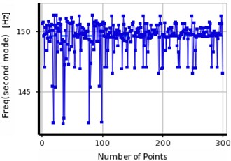
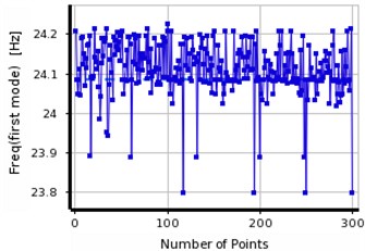
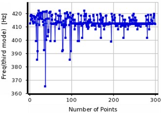
Fig. 15The convergence in the first three frequencies of steel beam using MMOGA
In MOGA, two out of three final responses have been fallen in same ranges which indicate the higher stability of analysis in MOGA. However, higher differences are observed between three final responses in MMOGA showing lack of stability in the analysis and subsequently low accuracy in the responses.
Comparison between three obtained results from MOGA and MMOGA, it is attempted to identify the final response. The first crack is located at 240 mm distance from the support with 4 mm depth. The damage location of the second crack was detected about 555 mm from the support with 6 mm depth. The validation procedure was verified based on the convergence between the OVS’s responses concentration and the actual location of the damage.
Table 6The obtained results from OVS before the last step of analysis in steel cantilever beam
Method | Crack position 1 (mm) | Crack position 2 (mm) | Natural frequency (Hz) | |||||||||
Distance | Depth | Distance | Depth | 1st mode | 2nd mode | 3rd mode | ||||||
OVS | E % | OVS | E % | OVS | E % | OVS | E % | |||||
MOGA | 1 | 233.05 | – | 3.89 | – | 556.01 | – | 6.29 | – | 24.084 | 149.788 | 412.261 |
2 | 148.79 | – | 6.50 | – | 569.65 | – | 6.29 | – | 24.093 | 149.866 | 412.839 | |
3* | 242.76 | 5.0 | 3.89 | 2.8 | 556.01 | 1.9 | 6.34 | 5.3 | 24.095 | 149.592 | 411.337 | |
MMOGA | 1 | 75.16 | – | 6.92 | – | 581.99 | – | 6.64 | – | 24.074 | 149.61 | 412.137 |
2* | 230.76 | 10.5 | 3.46 | 15.6 | 553.84 | 1.5 | 6.55 | 8.3 | 24.165 | 149.55 | 412.443 | |
3 | 385.78 | – | 7.33 | – | 588.07 | – | 6.64 | – | 24.187 | 149.63 | 412.49 | |
5.2. Specimen No. 2
The experimental information of Ref. [16] has been used as the output for proposed method in order to study the number of frequencies effective in the conducting research, the influence of decreasing the number of frequencies as well as support conditions. For this purpose, a specimen was selected with the cross section of 10 mm×10 mm, 400 mm length, 216 GPa modulus of elasticity and material mass density of 7650 kg/m3. Simply supported boundary conditions were selected for the beam. The location and depth of cracks are 80 mm and 5 mm, respectively, presented in Fig. 16.
In Table 7, experimental and numerical results of this beam are displayed in the third and fourth columns. The error value of 1.8 % observes in the results obtained from the first frequency due to the noise found during the experiment.
Table 7Natural frequencies in the two modes using numerical modeling and experimental results
Crack location (mm) | Natural frequency (Hz) | ||||||
Experimental method [16] | Numerical method (FEM) | Existing technique Ref. [16] | |||||
Position | Depth | 1st mode | 2nd mode | 1st mode | 2nd mode | 1st mode | 2nd mode |
80 | 5 | 24.044 | 149.268 | 24.086 | 149.660 | 23.962 | 148.660 |
Fig. 16The location and depth of crack in simply supported beam according to [16]
![The location and depth of crack in simply supported beam according to [16]](https://static-01.extrica.com/articles/16681/16681-img31.jpg)
![The location and depth of crack in simply supported beam according to [16]](https://static-01.extrica.com/articles/16681/16681-img32.jpg)
Table 7 tabulates the first and the second natural frequencies of steel beam based on three different methods including, experimental methods conducted by Ref. [16]; existing technique used by Ref. [16]; and numerical method accomplished by authors.
5.2.1. OVS responses using previous study according to [16]
In this section, the effect of number of modes on the convergence is studied based on the information presented in the previous sections. For this purpose, based on the experimental results, two natural frequencies are defined as the input for numerical method. The obtained results are evaluated using considered optimization methods (MOGA, MMOGA). Fig. 17 shows the convergence of the first and second frequencies towards the main response.
One important considerable point in using the experimental results is the amount of noises generated during experiment. The noises enter the results and make errors which may improperly influence the final response of OVS optimization process. The main reason of variation the convergence curves in Figs. 17 and 18 is the presence of noises which enter in the calculations while defining the input. The permanent existence of these noises indicates the execution capability of the proposed method (OVS).
Fig. 17Convergence process in the first two frequencies of steel beam using MOGA
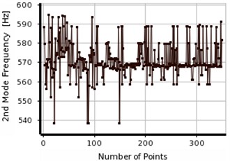
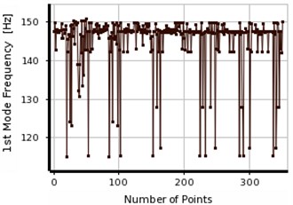
Fig. 18Convergence in the first two frequencies of steel beam using MMOGA
The responses were optimized based on MOGA and MMOGA as shown in Figs. 17 and 18, respectively. The process of response convergence is explained in each interval of population generation. According to Figs. 17 and 18, the population generation were scattered in the first and second frequencies. This fact is mainly due to the differences between numerical and experimental results, (Table 7). In the other words, the experimental results can be used as the input of optimization analysis for different numerical and experimental responses. However, changing in different frequencies due to different factors such as noises and measurement errors was the integral part of executions. Table 8 presents the final responses obtained from post-convergence analysis. According to this table, three results were extracted as the final responses, like previous scenarios. After the final evaluation, one response was defined as the optimal response which was unique in all cases. Therefore, it is not necessary to increase the number of the iterations in order to obtain the optimum responses. Maximum error level obtained in MOGA during optimization process was 1 %. The responses were evaluated, considering the limited information of input data (including first frequency of beam). Like previous scenarios, the accuracy of the calculated measurements increases as preliminary frequencies of structure increase. However, the responses seem to be acceptable concerning the limited available information.
The error level in MMOGA increases slightly due to population generation in optimization process. The final optimization results are isolated in both methods and presented in Table 8. According to Table 4, if two natural frequencies are considered as the input of the analysis, the concentration of the responses can be detected in both methods, (MOGA, MMOGA). For instance, in scenario No. 2, the obtained results were focused at the distance about 320 mm, which was not the actual location of the created crack. In order to, enhance the accuracy of the damage detection the numbers of the local optimal points were increased to five and seven points. However, the extra optimal locations were merged to the false answer. Therefore, using two natural frequencies as the input cannot be utilized to detect the exact location of the damage. Accordingly, the numbers of the inputs (natural frequencies of the beam) were increased to three ones, which lead to the exact location of the damage.
Table 8OVS results before the last step of analysis in steel cantilever beam
Method | Crack position (mm) | Natural frequency (Hz) | |||||
Distance | Depth | 1st mode | 2nd mode | ||||
Present study | E % | Present study | E % | ||||
MOGA | 1* | 80.76 | 1.0 | 5.02 | 1.0 | 147.39 | 568.28 |
2 | 322.20 | – | 5.02 | 1.0 | 148.04 | 563.46 | |
3 | 292.13 | – | 4.57 | 8.6 | 147.18 | 568.54 | |
MMOGA | 1* | 82.99 | 3.6 | 4.91 | 1.8 | 147.50 | 569.23 |
2 | 315.92 | – | 4.91 | 1.8 | 147.78 | 563.42 | |
3 | 372.9 | – | 7.19 | – | 148.49 | 568.17 | |
6. Numerical scenarios
In the previous scenarios, the aim of OVS was to verify optimum response. The efficiency of method was verified considering sufficient accuracies and optimal responses of all obtained results. Numerical scenarios were designed as the final stage to solve different problems of deep or semi-deep beams. Fig. 4 presents general procedure of solving problems for different support conditions. After conducting numerical analysis, a hypothetical zone was considered for the damage.
6.1. FEM modeling
In this scenarios, the beam was considered with modulus of elasticity of 200 GPa, material mass density of 7860 kg/m3 and Poisson’s ratio of 0.3 and studied for simply-supported, cantilever, clamped-clamped and simply-clamped conditions.
According to Fig. 19, the studied beam has 100 mm width, 200 mm height, 2000 mm length, and 10 ratio. The location of crack and its depth are 1000 mm and 100 mm, respectively.
Using numerical method, in Table 9, three natural frequencies of the beam for all conditions were displayed. Results in this table were used as the input for analysis in OVS. Maximum noise considered for solving problem was 1 %. In the following, results from proposed method (OVS) are studied.
Fig. 19A sample of support condition and crack location in the considered beam
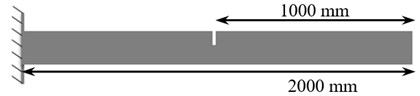
Table 9The obtained results of the first three natural frequencies using numerical method for all damaged beams
Row | Cantilever (Hz) | Clamped-clamped (Hz) | Simply supported (Hz) | Simple-clamped (Hz) |
1 | 38.83 | 224.07 | 94.89 | 157.1 |
2 | 200.55 | 634.78 | 440.35 | 531.6 |
3 | 655.16 | 1031.3 | 815.2 | 935.6 |
6.2. OVS responses using numerical analysis
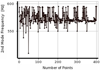
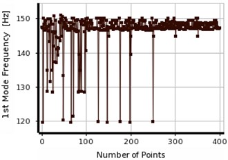
Considering the information represented in the previous scenarios, natural frequencies were considered as the analysis input. Then, the efficiency of OVS was evaluated through numerical scenarios. Finally, the error level was measured in the analysis. Figs. 20 and 21 present a sample investigation of the convergence process of responses for the cantilever beam. As an example, (Tables 10-12) and (Figs. 20 and 21) shows the results for numerical scenarios.
Table 10 displays the obtained results for a steel cantilever beam, considering two optimization methods (MOGA, MMOGA), showing high efficiency of the proposed method (OVS). Three final responses are considered in each method and after evaluation one final response is selected, concerning the conditions of the considered beam.
Fig. 20Convergence in the first three frequencies of steel cantilever beam using MOGA
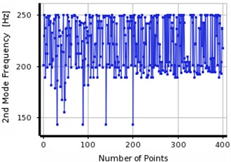
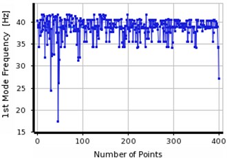
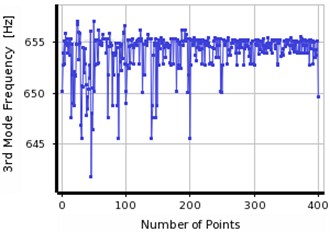
Table 10The results obtained from OVS before the final step of analysis in steel cantilever beam
Method | Crack position (mm) | Natural frequency (Hz) | ||||||
Distance | Depth | 1st mode | 2nd mode | 3rd mode | ||||
Present study | E % | Present study | E % | |||||
MOGA | 1* | 1016.43 | 1.5 | 103.8 | 3.6 | 38.37 | 197.56 | 655.03 |
2 | 920.11 | 8.6 | 109.1 | 8.3 | 38.85 | 189.12 | 652.89 | |
3 | 1851.26 | – | 45.39 | – | 38.82 | 242.21 | 654.64 | |
MMOGA | 1* | 1046.60 | 4.6 | 99.09 | 0 | 38.51 | 203.70 | 655.23 |
2 | 955.51 | 4.6 | 100.59 | 0.5 | 39.17 | 198.95 | 654.36 | |
3 | 1225 | 18.3 | 78.56 | – | 38.82 | 230.01 | 652.76 | |
Table 10 presents obtained results of the cantilever beam, considering the process of optimization analysis. The final results were briefly summarized in Tables 11 and 12. Table 11 presents the obtained results from proposed method, using MOGA, for different supports conditions. Maximum error level is lower than about 5 % in all conditions, indicating high accuracy of proposed method (OVS). It seems that, due to the boundary conditions, simply-clamped and simply-supported conditions contain some error. Therefore, the error levels increase due to the type of the support for the simply-supported beam. Such error may also occur in the numerical and experimental frequencies because of noise and measurement errors.
Fig. 21The convergence in the three frequencies of steel cantilever beam using MMOGA
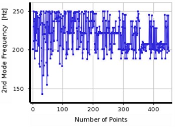
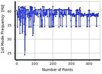
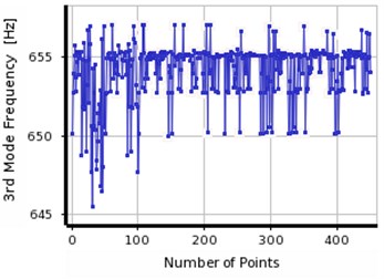
Table 11OVS results before the final step of analysis in steel beam with different support conditions using MOGA
Row |  |  |  |  | ||||||||
FEM (mm) | Present study (mm) | Error % | FEM (mm) | Present study (mm) | Error % | FEM (mm) | Present study (mm | Error % | FEM (mm) | Present study (mm) | Error % | |
1 | 38.83 | 38.37 | 1.1 | 224.07 | 224.06 | 0 | 94.89 | 93.58 | 1.4 | 157.1 | 157.80 | 0.4 |
2 | 200.55 | 197.56 | 1.4 | 634.78 | 643.75 | 0 | 440.35 | 437.87 | 0.5 | 531.6 | 537.82 | 1.1 |
3 | 655.16 | 655.03 | 0.1 | 1031.3 | 1031.45 | 0 | 815.2 | 815.51 | 0 | 935.6 | 936.82 | 0.1 |
Distance | 1000 | 1016.43 | 1.5 | 1000 | 992.74 | 0.7 | 1000 | 1056.60 | 5.3 | 1000 | 958.55 | 4.1 |
Depth | 100 | 103.8 | 3.6 | 100 | 99.95 | 0.7 | 100 | 103.67 | 3.5 | 100 | 93.06 | 6.9 |
Table 12 tabulates the obtained results from proposed method using MMOGA for boundary conditions. Maximum error level is 5 % in simply-supported, cantilever and clamped-clamped beams. This much is higher (11 %) in the simple-clamped beam. Comparing with the previous case, the errors level increases in this optimization method for all supports specifically for simply supported and simple-clamped beams.
The minimum numbers of input frequencies which were required to determine the damage location were investigated in another practical test. Accordingly, it was concluded that first three natural frequencies of deep beam can be sufficient. Having one frequency as an input in the optimization process, the error level was increased up to 90 % in all studied specimens. The final response of optimization process may lead to several different results in various locations with similar natural frequencies. To eliminate this issue the trial and error procedure would be a reasonable approach. Hence, at the very beginning of this study, the method was applied based on three final responses.
Table 12OVS results before the final step of analysis in steel beam with different supports conditions using MMOGA
Row |  |  |  |  | ||||||||
FEM (mm) | Present study (mm) | Error % | FEM (mm) | Present study (mm) | Error % | FEM (mm) | Present study (mm | Error % | FEM (mm) | Present study (mm) | Error % | |
1 | 38.83 | 38.51 | 0 | 224.07 | 223.72 | 0.2 | 94.89 | 93.43 | 1.5 | 157.1 | 154.69 | 1.5 |
2 | 200.55 | 203.70 | 1.5 | 634.78 | 643.35 | 1.3 | 440.35 | 440.21 | 0 | 531.6 | 523.48 | 1.5 |
3 | 655.16 | 655.23 | 0 | 1031.3 | 1030.58 | 0 | 815.2 | 808.66 | 0.8 | 935.6 | 928.89 | 0.7 |
Distance | 1000 | 1046.60 | 4.6 | 1000 | 982.07 | 1.7 | 1000 | 1002.69 | 0.2 | 1000 | 1027.43 | 2.6 |
Depth | 100 | 99.09 | 0 | 100 | 100.74 | 0 | 100 | 104.33 | 4.15 | 100 | 112.62 | 11.2 |
7. Conclusions
The main contribution of this research is to detect damages of structures based on the first three natural frequencies using OVS approaches. The natural frequencies were obtained for different structures using Modal Hammer test. In this study, it was attempted to determine the exact location of crack in the deep beams. For this purpose, FEM, MOGA, and MMOGA optimization methods were combined to provide a new convenient approach. The other purpose of this paper was to detect several cracks in different location of the beams. Accordingly, different experimental and numerical scenarios were presented to show the efficiency of the proposed method (OVS). The outcomes confirmed that the validity of the proposed method to detect damage in the structure. The obtained results demonstrated the convenience of the presented method to determine the location and depth of damages with the error of lower than about 5 % in all scenarios. Concerning the different support conditions illustrated that the more fixity at supports (clamped-clamped) leads to less errors measurement. The comparison between our experimental achievements and the results from the presented experimental scenarios by the others ([15] and [16]) indicated the sufficient accuracy of OVS for identifying the defective zone.
Regarding to the responses of two optimization methods, the results achieved from MMOGA showed higher accuracies for some scenarios. However, MOGA provided precise responses in the experimental and numerical scenarios. Nearly 95 % of the analysis results attained from two optimization methods revealed sufficient accuracies. Therefore, MOGA and MMOGA can be considered as complementary approaches. Which means, while MOGA cannot be reached to the optima responses, MMOGA can be resolved this issue. Based on the experimental observations, it was decided that the minimum numbers of frequencies inputs can be approximately equaled to the first three frequencies. However, using two methods can lead to eliminate some responses which may be far from the main frequencies and induce a mistake in the determination of the optimum response. The consumed time for optimization was recorded for both MOGA and MMOGA methods, concerning the final results and convergence to final response in OVS. The required time and memory space for MMOGA were less than MOGA, due to the data distribution of Kriging algorithm. The noises resulted from measurement errors, temperature; environmental vibrations and so on could bring the problem to achieve the final precise response. The noises generated in the numerical and experimental results were experienced 1 % and 2 % variation for the first and higher frequencies, respectively. Finally, it was evidenced that using OVS method can be considered as one of the proper methods to detect the location and depth of cracks with acceptable error.
References
-
Kourehli S. S., et al. Structural damage detection using incomplete modal data and incomplete static response. KSCE Journal of Civil Engineering, Vol. 17, Issue 1, 2013, p. 216-223.
-
Goldfeld Y., Elias D. Using the exact element method and modal frequency changes to identify distributed damage in beams. Engineering Structures, Vol. 51, 2013, p. 60-72.
-
Perera R., Marin R., Ruiz A. Static-dynamic multi-scale structural damage identification in a multi-objective framework. Journal of Sound and Vibration, Vol. 332, Issue 6, 2013, p. 1484-1500.
-
Seyedpoor S. A two stage method for structural damage detection using a modal strain energy based index and particle swarm optimization. International Journal of Non-Linear Mechanics, Vol. 47, Issue 1, 2012, p. 1-8.
-
Miguel L. F. F., Lopez R. H., Miguel L. F. F. A hybrid approach for damage detection of structures under operational conditions. Journal of Sound and Vibration, Vol. 332, Issue 18, 2013, p. 4241-4260.
-
Miguel L. F. F., et al. Damage detection under ambient vibration by harmony search algorithm. Expert Systems with Applications, Vol. 39, Issue 10, 2012, p. 9704-9714.
-
Esfandiari A., Bakhtiari-Nejad F., Rahai A. Theoretical and experimental structural damage diagnosis method using natural frequencies through an improved sensitivity equation. International Journal of Mechanical Sciences, Vol. 70, 2013, p. 79-89.
-
Mehrjoo M., Khaji N., Ghafory-Ashtiany M. Application of genetic algorithm in crack detection of beam-like structures using a new cracked Euler-Bernoulli beam element. Applied Soft Computing, Vol. 13, Issue 2, 2013, p. 867-880.
-
Su W., et al. Locating damaged storeys in a shear building based on its sub-structural natural frequencies. Engineering Structures, Vol. 39, 2012, p. 126-138.
-
Baghmisheh M. V., et al. A hybrid particle swarm-Nelder-Mead optimization method for crack detection in cantilever beams. Applied Soft Computing, Vol. 12, Issue 8, 2012, p. 2217-2226.
-
Zheng S.-J., Li Z.-Q., Wang H.-T. A genetic fuzzy radial basis function neural network for structural health monitoring of composite laminated beams. Expert Systems with Applications, Vol. 38, Issue 9, 2011, p. 11837-11842.
-
Meruane V., Heylen W. A hybrid real genetic algorithm to detect structural damage using modal properties. Mechanical Systems and Signal Processing, Vol. 25, Issue 5, 2011, p. 1559-1573.
-
Standard Test Method for Measuring the P-Wave Speed and the Thickness of Concrete Plates Using the Impact-Echo Method. American Society for Testing and Materials, ASTM C1383-04, USA, 2010.
-
Standard Test Method for Pulse Velocity Through Concrete. Annual Book of ASTM Standards, American Society of Testing Material, ASTM C597, 2009.
-
Ruotolo R., Surace C. Damage assessment of multiple cracked beams: numerical results and experimental validation. Journal of Sound and Vibration, Vol. 206, Issue 4, 1997, p. 567-588.
-
Yoon H.-I., Son I.-S., Ahn S.-J. Free vibration analysis of Euler-Bernoulli beam with double cracks. Journal of Mechanical Science and Technology, Vol. 21, Issue 3, 2007, p. 476-485.
-
Long-Fei W., Le-Yuan S. Simulation optimization: a review on theory and applications. Acta Automatica Sinica, Vol. 39, Issue 11, 2013, p. 1957-1968.
-
Hjelmstad K., Shin S. Crack identification in a cantilever beam from modal response. Journal of Sound and Vibration, Vol. 198, Issue 5, 1996, p. 527-545.
-
Koh B., Choi J., Jeong M. Damage detection through genetic and swarm-based optimization algorithms. International Conference on Engineering, Science, Construction and Operations in Challenging Environments, 2010.
-
Law S., Shi Z., Zhang L. Structural damage detection from incomplete and noisy modal test data. Journal of Engineering Mechanics, Vol. 124, Issue 11, 1998, p. 1280-1288.
-
Chung H.-S., Alonso J. J. Multiobjective optimization using approximation model-based genetic algorithms. AIAA Paper, 2004.
-
Jeong S., Murayama M., Yamamoto K. Efficient optimization design method using kriging model. Journal of Aircraft, Vol. 42, Issue 2, 2005, p. 413-420.
-
Li F., et al. Interval multi-objective optimisation of structures using adaptive Kriging approximations. Computers and Structures, Vol. 119, 2013, p. 68-84.
-
Li G., et al. Improving multi-objective genetic algorithms with adaptive design of experiments and online metamodeling. Structural and Multidisciplinary Optimization, Vol. 37, Issue 5, 2009, p. 447-461.
-
Weaver Jr W., Timoshenko S. P., Young D. H. Vibration Problems in Engineering. John Wiley and Sons, 1990.
-
Tada H., Paris P., Irwin G. The Analysis of Cracks Handbook. ASME Press, New York, 2000.
-
Petyt M. Introduction to Finite Element Vibration Analysis. Cambridge University Press, 2010.
-
Khaji N., Shafiei M., Jalalpour M. Closed-form solutions for crack detection problem of Timoshenko beams with various boundary conditions. International Journal of Mechanical Sciences, Vol. 51, Issues 9-10, 2009, p. 667-681.
-
Ostachowicz W. M., Krawczuk M. Analysis of the effect of cracks on the natural frequencies of a cantilever beam. Journal of Sound and Vibration, Vol. 150, Issue 2, 1991, p. 191-201.
-
Chen L. W., Chen C. L. Vibration and stability of cracked thick rotating blades. Computers and Structures, Vol. 28, Issue 1, 1998, p. 67-74.
-
Fayyadh M. M., Razak H. A., Ismail Z. Combined modal parameters-based index for damage identification in a beamlike structure: theoretical development and verification. Archives of Civil and Mechanical Engineering, Vol. 11, Issue 3, 2011, p. 587-609.
-
Srinivas V., Sasmal S., Ramanjaneyulu K., Antony Jeyasehar C. Influence of test conditions on modal characteristics of reinforced concrete structures under different damage scenarios. Archives of Civil and Mechanical Engineering, Vol. 13, Issue 4, 2013, p. 491-505.
-
Goszczyńska B., Świt G., Trąmpczyński W., Krampikowska A., Tworzewska J., Tworzewski P. Experimental validation of concrete crack identification and location with acoustic emission method. Archives of Civil and Mechanical Engineering, Vol. 12, Issue 1, 2012, p. 23-28.
About this article

