Simulation of rolling bearing vibration in diagnostics

1. Introduction

Rolling bearings are key elements in machines, and their reliability, thus their vibrations are an important issue [1-17]. Rolling bearings vibrations are parametric, because positions of rolling elements are the function of time, in spite of a certain slip. These vibrations are nonlinear, because the Hertzian contact is nonlinear. And thus, characteristics phenomena are observed: bistability, jump of amplitude, bifurcation directly leading to chaos, chaotic vibrations, and windows of periodic vibrations. These phenomena involve the relations clearance – amplitude and amplitude – clearance ambiguous. If, bistability or chaotic vibrations are observed, then for the same clearance, various magnitudes of amplitudes can be observed. It should be mentioned, that chaotic vibrations are non-periodic, which leads to non-recurrent results, in other words, dispersion obtained results. Whereas, bistability, bifurcation directly lead to chaos, and windows of periodic vibrations lead to jumps of amplitude. In consequence small changes of clearance, which are below 0.5 m, can lead to large changes of amplitude – jumps of amplitude. The aforementioned phenomena are simulated with numerical methods, because analytical methods are very difficult in this case [6, 7, 18]. Summarising, the contact introduces strong non-linearity even to very simple systems, and makes their vibrations sophisticated [19-21]. Most of articles present fragmentary studies on ball bearings vibrations, they are focused on one phenomenon, thus there is a need to present a study covering a wide range of clearance.

2. Model of rolling bearing

The deep groove ball bearing 608Z is modelled as a mechanical system (Fig. 1). First, the housing is modelled as a fixed rigid body. Next, the shaft is modelled as a rigid body, which have a mass and three degree of freedom. Shaft rotates, and vibrates in two directions $x$ and $y$. Then, balls and the Hertzian contacts are modelled as non-linear massless springs. Finally, the shaft and inner race rotate in counter-clockwise direction, thus balls circulate in the counter-clockwise direction. In consequence stiffness of bearing is a function of time which excite parametric vibrations.

The following forces act on the shaft: spring force, damping force, friction force, external force, and inertial force, they are described below. The spring forces $R_n$ are described by the following equations:

where: ${\delta }_n$ – is sum of contact deflections which correspond to $n$th ball, $d$ – represents diameter of balls m, $D_1$ – denotes diameter of inner race, $D_2$ – is diameter of outer race, $x_1$, $y_1$ – are displacement of shaft, $\alpha$ – denotes angular position of $n$th ball, $R_n$ – is contact force acting on $n$th ball $N$, and $K$ – is coefficient of contact stiffens N/m^1.5. The diameters of studied rolling beating were measured. A linear model describes the damping force. Components of damping force $F_d$ are described by the following equations:

where: $F_{dx}$ and $F_{dy}$ – are $x$ and $y$ components of the damping force N, $c$ – denotes coefficient of damping $c=$ 200 (Ns)/m. This model of damping was used previously. The friction force of rolling contact is described by the following expression:

where: $F_{otn}$ – denotes rolling friction force acting on $n$th ball, and $\mu$ – is coefficient of rolling friction. This is classical model of friction force. The external force $F$ is constant during simulation, and is presented in Table 1. The equations of motion in two directions are presented below:

where: $m$ – represents equivalent mass attached to shaft.

This idealised model of rolling bearing provides an opportunity to estimate amplitudes of vibrations and select state indicators, which is very useful in designing and machinery diagnostics; because computer simulation is very cheap comparing with experimental investigations. A key factor is clearance, thus vibrations are simulated for various magnitudes of clearance. Obtained results are presented below.

Fig. 1a) The deep groove ball bearing 608Z and b) its model [7]

a)

b)

3. Results of simulation of state indicators

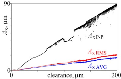
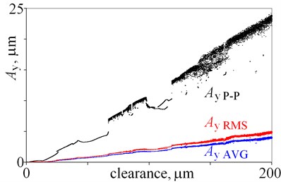
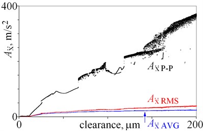
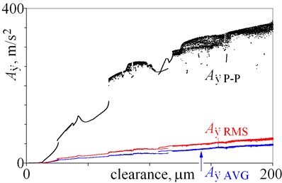
One of the simplest state indicators is amplitude of vibration. Three amplitudes, which are widely used in machinery diagnostics, are depicted against clearance in Figs. 2 and 3. They are described by the following equations:

where: $A_{xP-P}$ – denotes peak-to-peak amplitude, $x_{max}$ – is the largest magnitude, $x_{min}$ – represents the smallest magnitude, $A_{xRMS}$ – is root mean square amplitude, $x_{mean}$ – denotes arithmetic mean of $x$, $j$ – is the number of samples, whereas $A_{xAVG}$ – is average amplitude. The arithmetic mean is included in two equations because, in practice position of the origin is unknown. These amplitudes can be calculated for: displacement, velocity, acceleration, and two directions, which provides eighteen state indicators. These amplitudes should be described, and the best state indicators should be selected.

For small clearance, being from 0 to 12 m, amplitudes seem to be almost constant. Next, amplitudes generally rise, but local minima, jumps of amplitude, and bistability are observed. Then, for clearance, being larger than 66 m, chaotic motion is observed. Chaotic motion in Fig. 2 is represented by a number of points – a point cloud, because various results (amplitudes) are obtained for the same clearance. Dispersion obtained amplitudes is result of non-periodic, chaotic motion. If a line is below these points, it means that the window of periodical vibrations is observed; because amplitudes of periodic vibrations are usually smaller, than amplitudes of chaotic vibrations. Bifurcation diagram provides an opportunity to explain changes of amplitudes, which are associated with bifurcations.

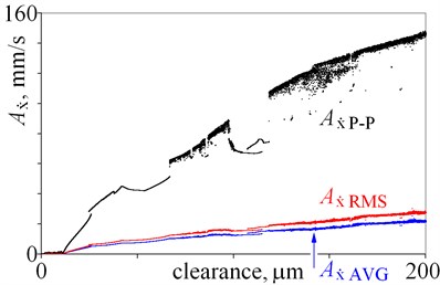
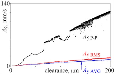
Presented results show, that the relation: clearance – amplitude and amplitude – clearance is ambiguous (Fig. 2). Nevertheless, amplitudes of displacement $A_{xRMS}$, $A_{xAVG}$, $A_{yRMS}$, $A_{yAVG}$ seems to be good state indicators, because of small local minima and small jumps of amplitude (Fig. 2(a), (b)). Moreover, average amplitude and root mean square amplitude are less sensitive to extreme values than peak to peak amplitude. Amplitude $A_{xP-P}$ is nearly proportional to clearance, which is an advantage. Jumps of amplitude and minima observed for $A_{yP-P}$ are relatively larger than one observed for $A_{xP-P}$, and amplitude $A_{yP-P}$ is smaller than $A_{xP-P}$. This leads to conclusion, that $A_{xP-P}$ is better state indicator than $A_{yP-P}$. Then, the results obtained for velocity are depicted in Fig. 2(c), (d). Minima and jumps observed for amplitudes of velocity $\dot{x}$ are larger than the ones observed for displacement $x$ (Fig. 2(a), (c)), thus displacement is a better state indicator. Whereas, graphs obtained for $y$ and $\dot{y}$ have similar shape (Fig. 2 (b), (d)). Finally, the results obtained for acceleration are depicted in Fig. 2(e), (f). Amplitudes generally rise with an increase of clearance but jumps of amplitude and local minima locally change this tendency. Amplitudes obtained for $\ddot{x}$ seem to be better state indicators than amplitudes obtained for $\ddot{y}$, because shapes of graphs are less complex. These conclusions are valid for clearance being from 0 to 200 m.

Fig. 2Amplitudes of vibrations against various magnitudes of clearance (0 do 200 m)

a)

b)

c)

d)

e)

f)

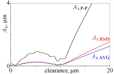
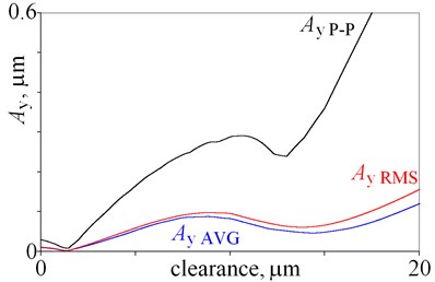
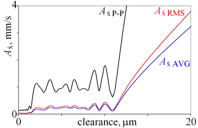
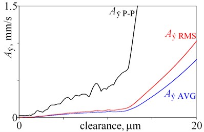
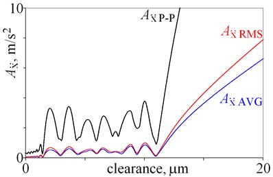
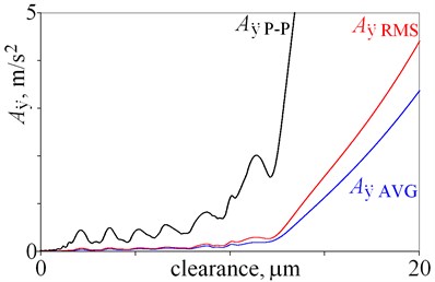
Amplitudes of vibrations are the smallest for clearance being below 12 m, thus this part is magnified in Fig. 3. Local minima are observed for amplitudes of displacement $A_{xP-P}$, $A_{xRMS}$, $A_{xAVG}$, $A_{yP-P}$, $A_{yRMS}$, and $A_{yAVG}$ in Fig. 3(a), (b), thus relation amplitude-clearance is ambiguous in this case. A number of local maxima are observed for $A_{\dot{x}P-P}$, $A_{\dot{x}RMS}$, $A_{\dot{x}AVG}$, and $A_{\ddot{x}P-P}$, $A_{\ddot{x}RMS}$, $A_{\ddot{x}AVG}$ in Fig. 3(c), (e). These maxima are result of resonances, thus amplitudes of velocity and acceleration obtained for $x$-direction are not the best state indicators. Better state indicators are amplitudes obtained for $\dot{y}$ and $\ddot{y}$, because amplitudes rise and local minima are smaller. Various state indicators are selected for a large clearance (Fig. 2) and a small clearance (Fig. 3), because graphs have various shapes within the studied ranges. This shows, that researchers can indicate various state indicators for various conditions e.g. clearance. Moreover, the obtained results lead to practical conclusion. If, small amplitudes of vibrations are required, then the clearance should be below 12 m, and hard coatings should be used. Hard coatings provide an opportunity to reduce the wear and extend the lifetime.

Fig. 3Amplitudes of vibrations obtained for clearance being from 0 do 20 m

a)

b)

c)

d)

e)

f)

Apart from amplitudes, impulse factor, crest factor, and waveform factor are used as state indicators. These factors are described by the following equations:

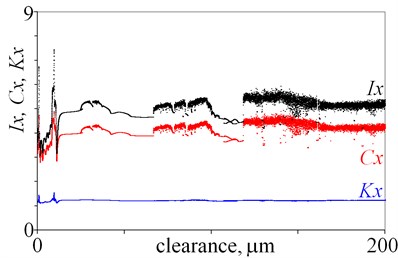
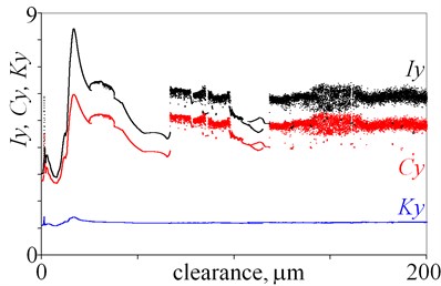
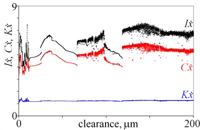
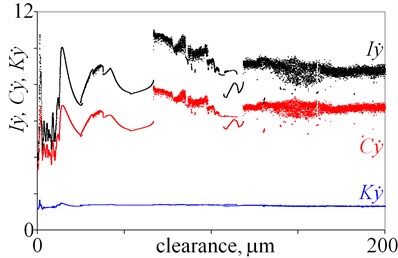
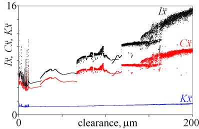
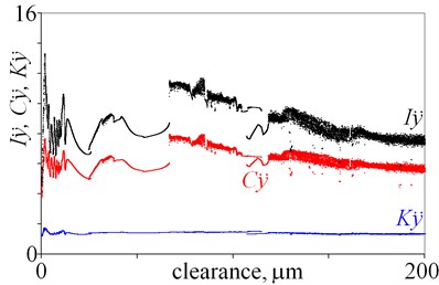
where: $I_x$ is impulse factor, $C_x$ denotes crest factor, and $K_x$ represents waveform factor. These factors can be calculated for: displacement, velocity, acceleration, and two directions, which give next eighteen state indicators. These state indicators are depicted in Fig. 4.

Fig. 4Impulse factor I, crest factor C, and waveform factor K obtained for displacement, velocity and acceleration against various magnitudes of clearance

a)

b)

c)

d)

e)

f)

As is evident from the obtained results, relations factor-clearance and clearance-factor are ambiguous. In Fig. 4(a) various values of factors are observed for a clearance being below 10 m. Then, jumps are observed for a clearance being 66.6 m and 118.2 m, which are associated with bifurcations. It is difficult to find any tendency, for example an increase of factors along with increasing clearance. Next, similar jumps of factors are observed in Fig. 4(b) for clearance being 66.6 m and 118.2 m. Moreover, maximal values of factors are observed for clearance being 16.5 m. After that, large dispersion of factors is observed in Fig. 4(c), (d), thus general tendency is difficult to find. Locally minima and maxima are observed, thus local tendency –increase or decrease can be found within small intervals. Whereas, factors $I_{\ddot{x}}$, $C_{\ddot{x}}$ and $K_{\ddot{x}}$ seem to be good state indicators, because they generally rise along with increasing clearance (Fig. 4(e)). Some variation of factors are observed for small a clearance, but it is observed for x direction. Finally, factors are calculated for $\ddot{y}$ (Fig. 4(f)). Values of factors change for a clearance being from 0 to 66.6 m, and thus many local minima and maxima are observed. But for a clearance being above 66.6 m values of factors generally drop. Summarising, the best factors are $I_{\ddot{x}}$, $C_{\ddot{x}}$ and $K_{\ddot{x}}$, nevertheless amplitudes seems to be better state indicators for the studied system.

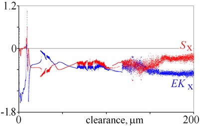
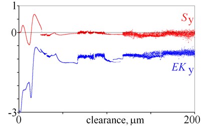
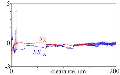
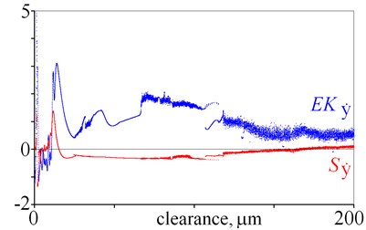
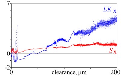
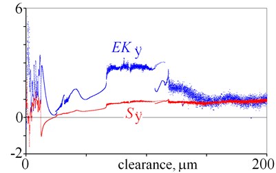
Fig. 5Excess kurtosis and skewness obtained for displacement, velocity and acceleration against various magnitudes of clearance

a)

b)

c)

d)

e)

f)

Next, excess kurtosis and skewness can be used as state indicators. They are described by the following equations:

where: $s$ – denotes standard deviation. Excess kurtosis and skewness can be calculated for displacement, velocity, acceleration and two directions, which gives twelve state indicators. They are depicted in Fig. 5. As it is evident from the obtained results, many local minima are observed, thus a general tendency is difficult to find. Nevertheless, excess kurtosis $E{K}_{\ddot{x}}$ depicted in Fig. 5(e) gets lager for rising clearance, which shows that is sensitive to clearance.

Summarising this section it should be mentioned, that selected amplitudes [8], factors obtained for $\ddot{x}$$I_{\ddot{x}}$, $C_{\ddot{x}}$, $K_{\ddot{x}}$ and excess kurtosis obtained for $\ddot{x}$$E{K}_{\ddot{x}}$ are good state indicators.

4. Bifurcation diagrams

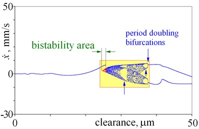
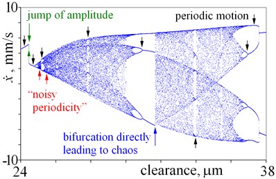
Bifurcation diagrams (Fig. 6) correspond to Fig. 2. First, periodical vibrations are observed (0-25.6 m), they are represented by a single line (Fig. 6(a)). Then, bistability area is observed, thus jumps of amplitude takes pace (Fig. 2(e) and 6(a), 7(a)).

Fig. 6Bifurcation diagrams obtained for various magnitudes of clearance

a)

b)

c)

d)

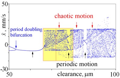
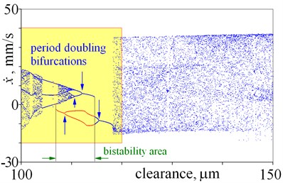
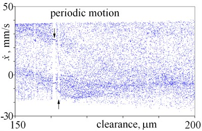
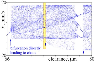
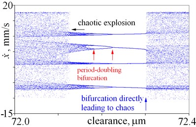
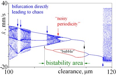
In this case, both periodical vibrations and chaotic vibrations can be obtained for the same clearance. Bifurcations directly leading to chaos, cascades of period-doubling bifurcations leading to chaos, “noisy periodicity” and windows of periodic motion are depicted in Fig. 6(a). Next, periodical vibrations are observed, which period is two times larger than period of excitation – double line (37.6-53 m) (Fig. 6(a), (b), 7(a)). After bifurcation (53 m), vibration period equals period of excitation (single line). After that, bifurcation directly leading to chaos is observed for a clearance being 66.6 m (Fig. 6(b) and 7(b)). This bifurcation significantly changes the amplitude, thus jump of amplitude is observed in Fig. 2(e), (f). It should be mentioned, that within large interval of chaotic motion, small windows of periodic vibrations are observed (66.6-100 m). Small window of periodic motion is magnified and depicted in Fig. 7(c), which shows: structure of this window, bifurcations and chaotic explosion. Lager windows of periodic motion are observed for clearance being near 78 m and 85 m (Fig. 6(b)). Some changes of amplitudes correspond to these windows of periodic motion (Fig. 2(e), (f)). Last, second bistability is observed (Fig. (6), (c) and 7(d)). Bifurcations directly leading to chaos, period-doubling cascade leading to chaos, “noisy periodicity”, jumps of amplitude, and opposing period-doubling bifurcations “bubble” are observed. Both periodic and chaotic vibrations can be exited for this bistability. It should be mentioned that, a local minima of amplitude corresponds to this bistability in Fig. 2. Finally, large interval of chaotic motion with small windows of periodic motion is observed (Fig. 6(c), (d)).

Summarising this, bifurcation diagram is necessary to explain changes of amplitudes, and should be used more often in machinery diagnostics.

Fig. 7Details of bifurcation diagrams obtained for various magnitudes of clearance

a)

b)

c)

d)

5. Conclusions

Relations of clearance-state indicators provide valid information for machinery diagnostic, because state indicators can be selected. For the studied example, amplitudes of displacement seem to be the best. Similar conclusion was presented in literature [8]. Moreover, factors obtained for $\ddot{x}$$I_{\ddot{x}}$, $C_{\ddot{x}}$, $K_{\ddot{x}}$ and excess kurtosis obtained for $\ddot{x}$$E{K}_{\ddot{x}}$ are good state indicators. Before expensive experimental studies, results of simulation can be analysed, which provide valid information and opportunity to reduce costs of experimental studies. Local minima and jumps of amplitudes, which introduce difficulties in machinery diagnostic, can be explained based on bifurcation diagrams. Local minima and jumps of amplitude make the relation of state indicator-clearance ambiguous. Finally, a number of nonlinear phenomena were observed for this model: bistability, jump of amplitude, opposing period-doubling bifurcations “a bubble”, period-doubling bifurcations leading to chaos, bifurcation directly leading to chaos, chaotic vibrations, windows of periodic vibrations, “noisy periodicity”, and chaotic explosion. This shows that linear models of rolling bearing can lead to large errors.