The experimental investigation of nonlinear impact behaviors of partial rolling bearing with failure collision

He, Xing; Wang, Qiang; Liu, Yongbao; Xu, Huidong; Liu, Shuyong

doi:10.21595/jve.2017.18149

Journal of Vibroengineering

Browse Journal

Submit article

Published: 30 June 2017

Check for updates

The experimental investigation of nonlinear impact behaviors of partial rolling bearing with failure collision

Xing He¹

Qiang Wang²

Yongbao Liu³

Huidong Xu⁴

Shuyong Liu⁵

^{1, 2, 3, 5}College of Power Engineering, Naval University of Engineering, Wuhan, Hubei 430033, P. R. China

²Department of Weaponry Engineering, Naval University of Engineering, Wuhan, Hubei 430033, P. R. China

⁴College of Mechanics, Taiyuan University of Technology, Taiyuan, Shanxi 030024, P. R. China

Corresponding Author:

Qiang Wang

Cite the article Download PDF

Downloads 1379

CrossRef Citations 1

Abstract

The influence of nonlinear impact behavior of partial failure collision rolling bearing is studied when the pitfall occurs in the inner ring. The piecewise non-smooth experiment model of three-degree-of-freedom rolling bearing system with fault in inner ring is established, and the experiment method is used to further reveal the bifurcations and chaos of bearing system through establishing the Poincaré mapping on the collision plane. The nonlinear impact behaviors are studied with the vibration force increasing, when the vibration frequency is determined. The impact signal spectrum characteristics are analyzed through changing the quality of the mass $M_{1}$ after adding a force sensor. The study of nonlinear impact behaviors of the fault bearing system provides reliable basis for the design and fault diagnosis and provides theoretical guidance and technical support for the actual design in the safe and stable operation of large high-speed rotating machinery.

1. Introduction

Bearing is one of the most important part of the rotating machinery and is widely used in aviation aircraft, spacecraft, rocket, ship, nuclear reactor and so on. It plays a key role for the safe running of the equipment. Once the bearing is broken, it will cause more serious consequences including security challenge and increasing downtime. The nonlinear vibration behaviors caused by fault are very complicated, which has significant effect on the design and fault diagnosis of bearing. Utkarshkumar Arvindbhai Patel et al. established the inner and outer ring fault mathematical model to research the nonlinear dynamic behavior of bearing fault according to Hertz contact theory. Because of the contact force and process exhibit nonlinear stiffness characteristic, the nonlinear behavior of the system can be analyzed through $n$ -dimension nonlinear simultaneous equations and numerical simulation [1]; N. Tandon and A. Choudhury studied the impact of the bearing by assuming different shape signals, such as sine wave, square wave and triangle wave respectively in the bearing inner ring and outer ring, rolling elements and the accuracy of the numerical simulation is proved by comparing the signal frequency response of the simulation and experimental data [2]; N. Tandon et al. described the fault characteristics through the frequency spectrum characteristics by considering the rolling bearing as a three degree of freedom fault model which is consisted of inner and outer ring raceway waviness, size irregular rolling body and so on [3]; N Sawalhi and R. B. Randall analyzed the process of rolling element in and out of fault location and studied the vibration of the bearing behavior pricewise by assuming the fault position signal as a step type which stirs up a more broad band frequency response and the cestrum analysis method is used to determine the fault location and fault type [4]; Alireza Moazenahmadi et al. [5] studied impact type and the signal response of the fault signal by establishing the failure nonlinear dynamic bearing model and assuming the fault is the rectangular shape with the size of the fault changing from small to large; He et al. [6] studied the dynamics of rolling bearing system with gaps under variable load. Zhang et al. [7] investigated the nonlinear dynamic characteristics and stability of rolling bearing system under the influence of non-equilibrium force. Tang et al. [8] obtained the nonlinear bearing force in work situation based on Hertz elastic contact theory and the kinesiology of rolling bearing, and analyzed vibration features of rolling bearing system. Gao et al. [9] established the dynamical equations of the spindle system based on Hertz contact force model and studied mechanism and pathway of the instability.

The rolling bearing with failure may be categorized into vibro-impact systems. The strong nonlinear characteristic caused by instantaneity and discontinuity of impact can exhibit rich dynamic behavior. Many researchers have investigated the bifurcation and chaos of vibro-impact systems by theoretical and numerical analyses. Shaw and Holmes [10] studied the oscillator system with single piece rigid constraint under the action of a harmonic force by using modern dynamics theoretical methods and analyzed the bifurcation behaviors of periodic motions by using center manifold and normal formal theory. Jin and Hu [11] studied the vibro-impact response of Hertz contact model of flexible beam system in theory and carried on the corresponding experiment verification. Luo and Xie [12] studied the complexity co-dimension-two bifurcation behaviors of a two-degree-of-freedom vibro-impact system. Ding and Xie [13] studied the path from torus bifurcations to chaos in a three-degree-of-freedom vibro-impact system. Jin and Lu [14] studied the Lyapunov exponent of vibro-impact system with constraining stops through building compound map and obtained the determinant indexes to differentiate periodic motion and chaos. Yue et al. [15] studied the co-dimension-two bifurcation and chaos of symmetric period motion in a three-degree-of-freedom vibro-impact system and pointed out that symmetry can suppress some kinds of bifurcations of system.

Though these researches acquire many achievements, most of the researches center on theoretical and numerical analyses of dynamical behaviors in the rolling bearing with failure. This paper studies the dynamic behavior of partial rolling bearing with failure collision via experiment. The design of the testing rig and experimental procedures are described in detail. The rich dynamical behaviors are revealed by changing excitation frequencies.

2. The theoretical model design

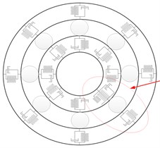
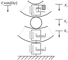
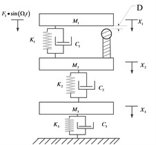
The three-degree-of-freedom vibro-impact physical model of rolling element bearing with fault in inner ring is shown in Fig. 1, in it (a) is the whole bearing with failure, (b) is the particle rolling bearing with failure collision, (c) is the experimental simplified figure of partial rolling bearing with failure collision. The purpose is to study the nonlinear behaviors of partial rolling bearing with failure collision, and the Fig. 1(c) is designed to make sure the collision is point collision to simulate the collision in real bearing.

Fig. 1The three-degree-of-freedom vibro-impact model of bearing

a)

b)

c)

If there is only small fatigue pitfall on the inner ring, the system is described as rigid impact when the rolling elements pass through this fault location. The three-degree-of-freedom dynamic model with gap between $M_{1}$ and $M_{2}$ is shown in Fig. 1, in which, $M_{1}$ , $M_{2}$ , $M_{3}$ are equivalent mass block of shaft with inner ring, rolling elements and outer ring with base coordinate respectively. The corresponding vertical displacements are $X_{1},$ $X_{2}$ and $X_{3}$ respectively. The damping coefficients are $C_{1}$ , $C_{2}$ and $C_{3}$ , the stiffness parameters are $K_{1}$ , $K_{2}$ and $K_{3}$ . The exitation force is $F_{1} s i n (Ω_{1} t)$ acting on $M_{1}$ , $Ω_{1}$ is the revolution frequency of the shaft. The gap between $M_{1}$ and $M_{2}$ in the vibration system is D, and the recovery coefficient is $R$ . When the relative displacement between the $M_{1}$ and $M_{2}$ is more than $D$ , the rigid collision occurs.

3. Design of the experimental rig

3.1. The design of springs

The spring is one of the most important component in the experiment. The material used is 65 Mn, and the parameters designed of the three kinds of springs are in Table 1. In order to be convenient to install, the design of the spring is set to lap two coils up and down respectively, so the total number of coils is 4 more than the working coils.

(1) Allowable shearing stress $[τ]$ (kg/mm²) of the spring is classified with three classes, I, II and III. The stress values are 0.3 $σ_{b}$ , 0.4 $σ_{b}$ , 0.5 $σ_{b}$ respectively. Stress $σ_{b}$ is 130 (kg/mm²) when the steel wire diameter $d$ is 6 mm.

(2) The shear modulus $G$ (N/m²) and the modulus of elasticity E (N/m²). When the diameter $d$ of the steel wire is $4 \geq d \geq 0.5$ (mm), the range of G is 8300-8000 (N/m²), and $E$ is 20750-20500 (N/m²), while $d > 4$ (mm), the value of $G$ is 8000 (N/m²), and $E$ is 20000 (N/m²).

(3) Spring index $C$ , $C = D_{2} / d$ , where $D_{2}$ is the mean diameter of the coil.

(4) Spring curvature $K$ , $K = (4 C - 1) / (4 C - 4) + (0.615 / C)$ .

(5) Effective coils $n$ , $n = F_{n} G d^{4} / 8 P_{n} D_{2}^{3}$ .

(6) Spring stiffness $P^{'}$ , $P^{'} = G d^{4} / 8 D_{2}^{3} n$ .

(7) Gap between coils, $δ_{1}$ , $δ_{1} \geq 0.1 d$ .

(8) Pitch of spring $t = d + F_{j} / n + δ_{1}$ , generally, $t \approx D_{2} / 3$ - $D_{2} / 2$ , and space of coils is $δ = t - d$ .

(9) Free height of spring $H_{0} = n * t + 3.5 d$ .

Table 1The designed parameters of the three kinds of springs

Spring type	Type I	Type II	Type III
Outer diameter of spring	36 mm	33.9 mm	40.3 mm
Steel wire diameter	6 mm	6 mm	6 mm
Spring stiffness	8 kg/mm	12 kg/mm	4 kg/mm
Working coils	6 coils	5 coils	8 coils
Total number of coils	10 coils	9 coils	12 coils
Spring natural length	81 mm	71 mm	105 mm
Maximal load	140.234 kg	147.47 kg	126.57 kg
Maximal stroke	17.529 mm	12.357 mm	31.528 mm
Working stroke	10 mm	10 mm	10 mm

3.2. Measurement of the spring stiffness

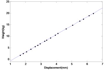
The stiffness values of springs are measured in lab. The designed theoretical values of the springs are $k_{1} =$ 8 kg/mm, $k_{2} =$ 12 kg/mm, $k_{3} =$ 4 kg/mm. The spring force versus displacement curves are shown in Figs. 2, 3 and 4. The stiffness values are calculated from the slope of the curves. The slopes of this lines are $k_{1} =$ 7.1270 kg/mm, $k_{2} =$ 12.3905 kg/mm, $k_{3} =$ 3.8927 kg/mm. The unit kg/mm is transformed into N/m, and we can get that the stiffness of the springs are $k_{1} =$ 69845 N/m, $k_{2} =$ 121427 N/m, $k_{3} =$ 38148 N/m, which are used in the following experiment.

Fig. 2The diagram of the weight and the deformation of Spring 1

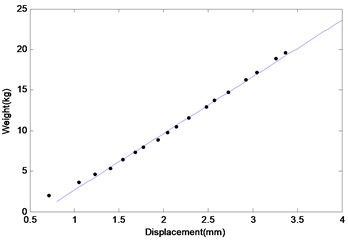
Fig. 3The diagram of the weight and the deformation of Spring 2

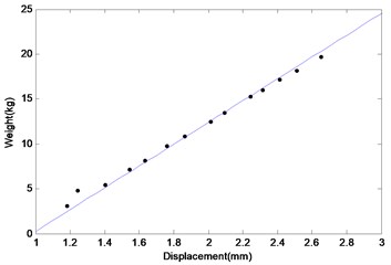
Fig. 4The diagram of the weight and the deformation of Spring 3

3.3. Components of the experimental rig

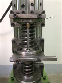
The experimental rig is composed of springs, collision ball, signal generator, data acquisition system, as shown in Fig. 5. A part of magnified figure is shown in Fig. 6. The collision structure comprises three mass blocks, the $M_{1}$ , $M_{2}$ and $M_{3}$ , and the springs $K_{1}$ , $K_{2}$ and $K_{3}$ . The linear rails which are vertical to the base are applied to ensure the mass blocks slide freely on the road. The collision part is designed between the $M_{1}$ and $M_{2}$ , and the gap between the $M_{1}$ and collision ball is $D$ , as shown in Fig. 7.

Fig. 5The experimental rig figure: (1) is the vibration generator, (2) is the collision test bench, (3) is the foundation bed, (4) is the guide rail

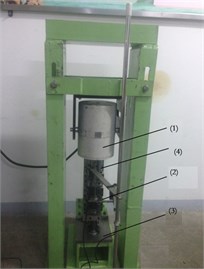
Fig. 6The partial magnified figure of the main body of the experimental bench: (1) is the laser displacement sensor, (2) is the mass block M1, (3) is the mass block M2, (4) is the mass block M3, (5) is the spring k1, (6) is the spring k2, (7) is the spring k3, (8) is the force sensor

The partial magnified figure of the main body of the experimental bench: (1) is the laser displacement sensor, (2) is the mass block M1, (3) is the mass block M2, (4) is the mass block M3, (5) is the spring k1, (6) is the spring k2, (7) is the spring k3, (8) is the force sensor

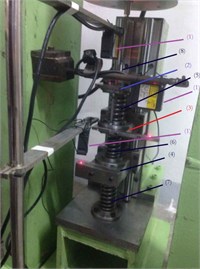
Fig. 7The collision position setting: (1) is the collision point

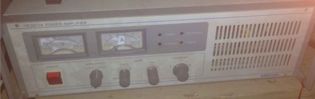
The force sensor is installed to connect the mass block $M_{1}$ and the vibration generator. The base is heavy enough to ensure its stability without vertical displacement when the collision occurs. The signal generator shown in Fig. 8 generates sinusoid, triangle, rectangular waveform. The power amplifier is shown in Fig. 9. Three laser displacement sensors whose linear accuracies are 5 um are applied to measure the vertical displacement of $M_{1}$ , $M_{2}$ and $M_{3}$ . The force sensor is used to obtain the excitation force curves and the type of multi-channel data acquisition system is the NI PXIE-1062Q.

Fig. 8The signal generator

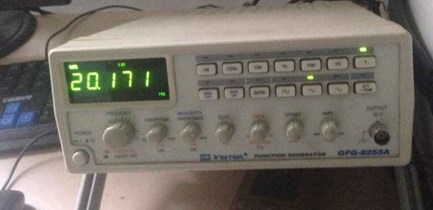
Fig. 9The power amplifier for exciter

4. Experiment study of the bifurcation and chaos responses in the system

4.1. The influence of increasing excitation force on the system

The chaotic response of the three-degree-of-freedom impact collision system under different excitation amplitude and constant frequency is researched in the section. The mass of the blocks are $M_{1} =$ 1.370 kg, $M_{2} =$ 1.700 kg, $M_{3} =$ 3.260 kg, respectively, and their test stiffness values are $K_{1} = k_{1} =$ 69845 N/m, $K_{2} = k_{2} =$ 121427 N/m, $K_{3} = k_{3} =$ 38148 N/m. The gap $D$ between $M_{1}$ and the top of the collision ball is 1.96 mm at the stationary state.

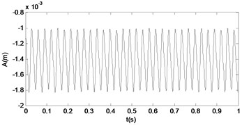
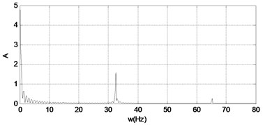
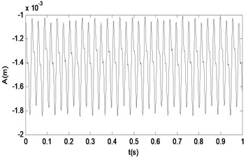
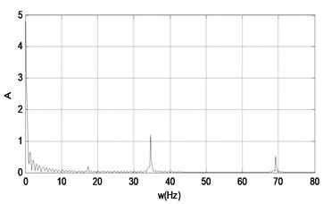
When the excitation frequency is 34.59 Hz, the power amplifier gain is adjusted to increase the amplitude of the excitation force, and the response is observed. When the gain is 0.5, the system response of $M_{1}$ is shown in Fig. 10 and Fig. 11.

When the power amplifier gain is 0.65, the response is shown in Fig. 12 and Fig. 13.

Fig. 10The time response and the signal spectrum diagram of M2

a)

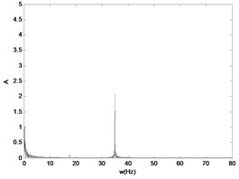
b)

Fig. 11The reconstructed phase diagram of M2

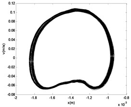
Fig. 12The time response and the signal spectrum diagram of M2

a)

b)

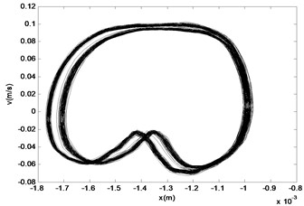
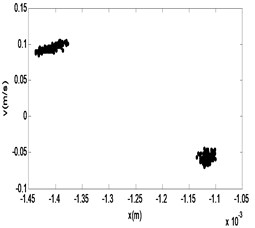
Fig. 13The phase diagram and Poincaré section of M2

a)

b)

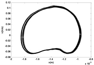
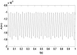
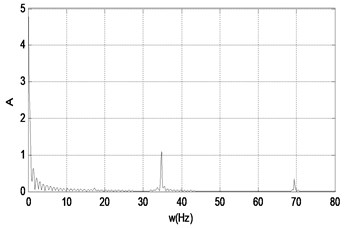
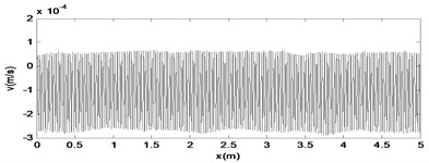
When the power amplifier gain is increased continuously to 1.7, the system response of $M_{2}$ is shown in Fig. 14 and Fig. 15.

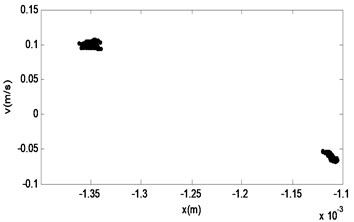
When the amplifier gain is increased continuously to 1.8, the system response of $M_{2}$ is shown in Fig. 16 and Fig. 17.

From the Figs. 10-17, we can see that the nonlinear behaviors occur in the system with the excitation force increasing when the frequency of the excitation is kept as a constant. When the force is small, that is the amplifier gain is 0.5, the system is in the stable period-1 motion initially, and we can see it in the reconstructed phase diagram of $M_{2}$ in Fig. 11, and the time response and the signal spectrum diagram is shown in Fig. 10. When the power amplifier gain is increased gradually and passes through the bifurcation point, the period-2 motion appears, just like the power amplifier gain is 0.65 which is near the critical gain, the period doubling bifurcation occurs. The phase diagram and Poincaré section of $M_{2}$ is shown in Fig. 13, and we can see that there is a little gap in the phase diagram, and the Poincaré mapping appears two points, from which we can fix it that the system is in stable period-2 motion. With the increasing of the amplifier gain, the gap is increasing in the phase diagram of $M_{2}$ in Fig. 15, and the Poincaré section of it appears two points, and the time response and the signal spectrum diagram of $M_{2}$ at the gain is in Fig. 14. When the amplifier gain is increased continuously to 1.8, the period-4 motion of the system appears. There are four mainly points in the Poincaré section of $M_{2}$ in Fig. 17. The amplitude of signal spectrum diagram of the system is changing in Fig. 10, Fig. 12, Fig.14, and Fig. 16. It is interesting that the attractor and Poincaré section of the reconstructed attractor is more sensitive to the change of the force than the spectra diagram.

Fig. 14The time response and the signal spectrum diagram of M2

a)

b)

Fig. 15The phase diagram and Poincaré section of M2

a)

b)

Fig. 16The time response and the signal spectrum diagram of M2

a)

b)

According to the analysis above, the system is in the stable period-1 motion initially, and with the decreasing of the amplifier gain, the critical bifurcation point appears, and then the period-2 motion and the period-4 motion of the system appear.

Fig. 17The phase diagram and Poincaré section of M2

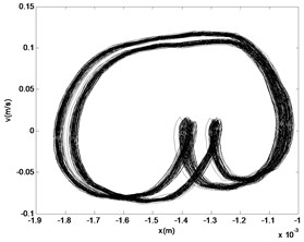
a)

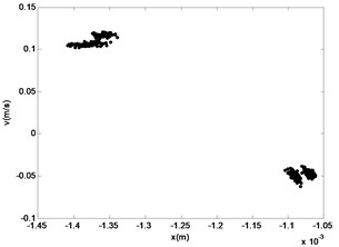
b)

4.2. The influence of increasing excitation force of the system after increasing the mass of $M_{1}$

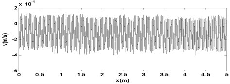
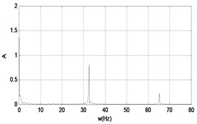
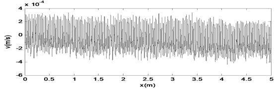
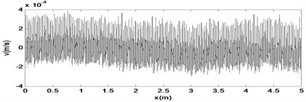
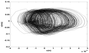
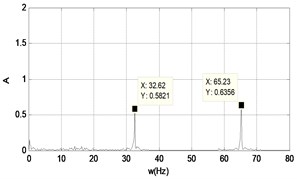
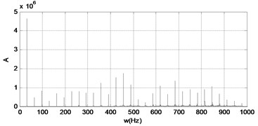
The force sensor is added to connect the exciter and the mass $M_{1}$ and the mass $M_{1}$ is increasing to $M_{1} =$ 1.475 kg, and the other parameters remain the same. The variation of the spectrum structure is researched from the force waveform signal. The excitation frequency is fixed at 32.6 Hz, the bifurcation behavior is observed. When the power amplifier gain is 0.5, the system has a single periodic motion, and the response diagrams of $M_{2}$ are shown in Fig. 18.

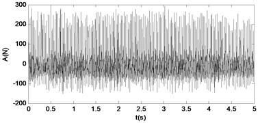
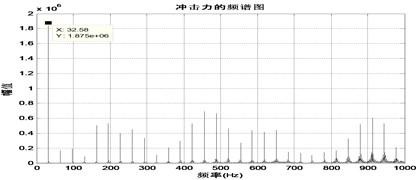
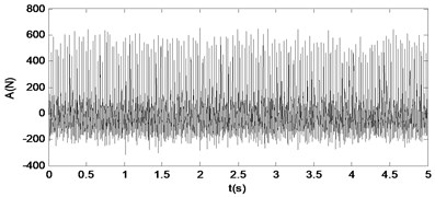
The spectrum and time response diagrams of the force are shown in Fig. 19. The collision frequency is the same as the exciter frequency in the single periodic state, which means the spectral characteristic is confirmed by experimental data.

Fig. 18The time response diagram, the phase diagram and the signal spectrum diagram of M2

a)

b)

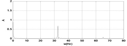
c)

Fig. 19The time response diagram and the signal spectrum diagram of force

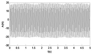
a)

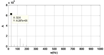
b)

When the gain is increased to 1.0, there is a deformation on the collision point, and the time response diagram, the phase diagram and the signal spectrum diagram of $M_{2}$ are shown in Fig. 20. The time response and the signal spectrum diagrams of force are shown in Fig. 21.

When the frequency 32.6 Hz, and the gain is increased to 1.2, the bifurcation behavior $M_{2}$ occurs, and the responses are shown in Fig. 22, from which we can see the bifurcation behaviors of the system. The corresponding dynamical force time series and spectrum are shown in Fig. 23.

Fig. 20The time response diagram, the phase diagram and the signal spectrum diagram of M2

a)

b)

c)

Fig. 21The time response diagram and the signal spectrum diagram of force

a)

b)

Fig. 22The time response diagram, the phase diagram and the signal spectrum diagram of M2

a)

b)

c)

When the frequency keeps constant, and the amplitude of force is increased further to 1.7, the bifurcation occurs clearly, and the responses are shown in Fig. 24. The corresponding dynamical force time series and spectrum are shown in Fig. 25.

Fig. 23The time response diagram and the signal spectrum diagram of force

a)

b)

Fig. 24The time response diagram, the phase diagram and the signal spectrum diagram of M2

a)

b)

c)

Fig. 25The time response diagram and the signal spectrum diagram of force

a)

b)

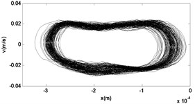
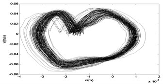
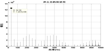
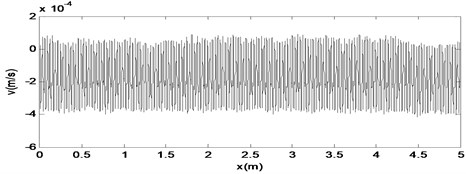
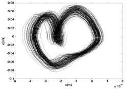
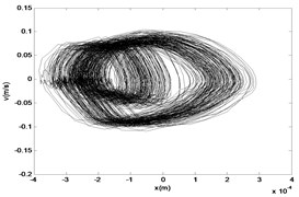
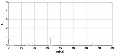
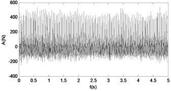
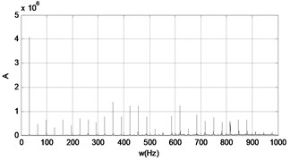
When the amplifier gain is increased further to 2.0, the chaotic vibration is obtained, and the phase attractor, time series, and spectrum are observed, as shown in Fig. 26. The corresponding dynamical force time series and spectrum are shown in Fig. 27.

According to the research, it is obvious that when the force sensor is added, the mass of $M_{1}$ is increased to $M_{1} =$ 1.475 kg, the chaotic response of the system changes as well. When the force amplitude increases, the system behaviors varies from the single periodic motion to the double periodic and chaotic vibration. The peak of the 2X spectrum also increases, as shown in Figs. 18, 20, 22, 24, 26. When the frequency is invariant, the peak of the harmonics varies slowly, as shown in Figs. 19, 21, 23, 25, 27. The response is very different from the responses in section 3.1, and we can see that the change of the quality parameters of the system will have a huge impact on the nonlinear behavior of the system.

Fig. 26The time response diagram, the phase diagram and the signal spectrum diagram of m2

a)

b)

c)

Fig. 27The time response diagram and the signal spectrum diagram of force

a)

b)

5. Conclusions

The experimental rig of three-degree-of-freedom bearing local fault simulation system is designed, and the nonlinear behaviors of the system are researched with the variation of the excitation force and mass of the block. Results show that when the excitation frequency keeps constant, the system exhibits the single periodic motion, double bifurcation and period-4 response with the increasing of the force amplitude. When the force sensor is installed, both the block mass and the bifurcation dynamical characteristic are changed. The single period, period-2 and chaotic response are obtained. The displacement, force time series and spectrum diagram are analyzed. It is discovered that the main frequency peak of the response is changed when the force amplitude is increased, even if the excitation frequency keep constant, which means the complexity of the vibro-impact system.

References

Patel Utkarshkumar Arvindbhai, Upadhyay Sanjay H. Theoretical model to predict the effect of localized defect on dynamic behavior of cylindrical roller bearing at inner race and outer race. Journal of Multi-Body Dynamics, 2014, p. 1-20.

Publisher
Tandon N., Choudhury A. An analytical model for the prediction of the vibration response of rolling element bearings due to a localized defect. Journal of Sound and Vibration, Vol. 205, Issue 3, 1997, p. 275-292.

Publisher
Tandon N., Choudhury A. A theoretical model to predict the vibration response of rolling bearings in a rotor bearing system to distributed defects under radial load. Journal of Tribology, Vol. 122, 2000, p. 609-614.

Publisher
Sawalhi N., Randall R. B. Vibration response of spalled rolling element bearings: Observations, simulations and signal processing techniques to track the spall size. Mechanical Systems and Signal Processing, Vol. 25, 2011, p. 846-870.

Publisher
Moazenahmadi Alireza, Petersen Dick, Howard Carl A nonlinear dynamic model of the vibration response of defective rolling element bearings. Proceedings of Acoustics, Vol. 17, 2013, p. 1-7.

Search CrossRef
He Z. X., Gan H. The study of rolling system dynamics behavior including the bearing shaft clearance. Journal of Vibration and Shock, Vol. 28, Issue 9, 2009, p. 120-124.

Search CrossRef
Zhang W. G., Gao S. H., Long X. H., Meng G. Nonlinear analysis for a machine-tool spindle system supported with ball bearing. Journal of Vibration and Shock, Vol. 27, Issue 9, 2008, p. 72-75.

Search CrossRef
Tang Y. B., Gao D. P., Luo G. H. Non-Linear bearing force of the rolling ball bearing and its influence on vibration of bearing system. Journal of Aerospace Power, Vol. 21, Issue 2, 2006, p. 366-373.

Search CrossRef
Gao S. H., Long X. H., Meng G. Three types of bifurcation in a spindle-ball bearing system. Journal of Vibration and Shock, Vol. 28, Issue 4, 2009, p. 59-63.

Search CrossRef
Shaw S. W., Holmes P. J. A periodically forced impact oscillator with large dissipation. International Journal of Applied Electromagnetics and Mechanics, Vol. 50, 1983, p. 849-857.

Publisher
Jin D. P., Hu H. Y., Wu Z. Q. Analysis of vibro-impacting flexible beams based on Hertzian contact model. Journal of Vibration of Engineering, Vol. 11, 1998, p. 46-51.

Search CrossRef
Luo G. W., Xie J. H. Bifurcation and chaos in a system with impacts. Physica D, Vol. 148, 2001, p. 183-200.

Publisher
Ding W. C., Xie J. H. Torus T² and its routes to chaos of a vibro-impact system. Physics Letters A, Vol. 349, 2006, p. 324-330.

Publisher
J. L., Lu Q. S., Wang Q. Calculation methods of floquet multipliers for non-smooth dynamic system. Chinese Journal of Applied Mechanics, Vol. 21, 2004, p. 21-26.

Search CrossRef
Yue Y., Xie J. H. Symmetry and bifurcations of a two-degree-of-freedom vibro-impact system. Journal of Sound and Vibration, Vol. 314, 2008, p. 228-245.

Publisher

Cited by

Dynamic analysis of localized defects in rolling bearing systems

Mengmeng Song | Shungen Xiao | Lixia Huang | Wanxiang Li

(2017)

About this article

Received

02 January 2017

Accepted

30 March 2017

Published

30 June 2017

SUBJECTS

Fault diagnosis based on vibration signal analysis

DOI

https://doi.org/10.21595/jve.2017.18149

Keywords

bearing

nonlinear behavior

collision

Poincaré mapping

Acknowledgements

The research is supported by the naval University of Engineering Ph.D. Innovation Funding (XYBJ1502) and the National Science Foundation of China (51579242) and the foundation No. 425517K143.

Author Contributions

Qiang Wang put forward the theme and idea of this manuscript and wrote this manuscript. Yongbao Liu conducted the simulation. Huidong Xu determined the experiment scheme. Shuyong Liu help to build the experimental platform. Xing He conducted the experimental data.

This is an open access article distributed under the Creative Commons Attribution License, which permits unrestricted use, distribution, and reproduction in any medium, provided the original work is properly cited.

Previous article in issue Previous Next article in issue Next

Research article

2024 02 29

Dynamic modeling and analysis of rolling bearing faults under time-varying excitations considering defect deformation

Chao Zhang, Yangbiao Wu, Shuai Xu, Feifan Qin, Le Wu, Bing Ouyang

Research article

2022 01 31

Fault identification and remaining useful life prediction of bearings using Poincare maps, fast Fourier transform and convolutional neural networks

Aditya Majali, Advait Mulay, Venugopalan Iyengar, Aniruddha Nayak, Pravin Singru

Research article

2018 02 15

Bearing failure prediction using Wigner-Ville distribution, modified Poincare mapping and fast Fourier transform

Pravin Singru, Vishnuvardhan Krishnakumar, Dwarkesh Natarajan, Ayush Raizada

Research article

2017 12 31

Effects of misalignment on the nonlinear dynamics of a two-shaft rotor-bearing-gear coupling system with rub-impact fault

Xin Lu, Junhong Zhang, Liang Ma, Jiewei Lin, Jun Wang, Jie Wang, Huwei Dai

X. He, Q. Wang, Y. Liu, H. Xu, and S. Liu, “The experimental investigation of nonlinear impact behaviors of partial rolling bearing with failure collision,” Journal of Vibroengineering, Vol. 19, No. 4, pp. 2598–2610, Jun. 2017, https://doi.org/10.21595/jve.2017.18149

Copy Extrica

Copied to clipboard!

TY  - JOUR
DO  - 10.21595/jve.2017.18149
UR  - https://doi.org/10.21595/jve.2017.18149
TI  - The experimental investigation of nonlinear impact behaviors of partial rolling bearing with failure collision
T2  - Journal of Vibroengineering
AU  - Wang, Qiang
AU  - He, Xing
AU  - Liu, Yongbao
AU  - Xu, Huidong
AU  - Liu, Shuyong
PY  - 2017
DA  - 2017/06/30
PB  - JVE International Ltd.
SP  - 2598-2610
IS  - 4
VL  - 19
SN  - 1392-8716
ER  - 

Copy Ris

Copied to clipboard!

@article{Wang_2017,
	doi = {10.21595/jve.2017.18149},
	url = {https://doi.org/10.21595/jve.2017.18149},
	year = 2017,
	month = {jun},
	publisher = {{JVE} International Ltd.},
	volume = {19},
	number = {4},
	pages = {2598--2610},
	author = {Qiang Wang and Xing He and Yongbao Liu and Huidong Xu and Shuyong Liu},
	title = {The experimental investigation of nonlinear impact behaviors of partial rolling bearing with failure collision},
	journal = {Journal of Vibroengineering}
}

Copy Bibtex

Copied to clipboard!

[1]Q. Wang, X. He, Y. Liu, H. Xu, and S. Liu, “The experimental investigation of nonlinear impact behaviors of partial rolling bearing with failure collision,” Journal of Vibroengineering, vol. 19, no. 4, pp. 2598–2610, Jun. 2017, doi: 10.21595/jve.2017.18149.

Copy IEEE

Copied to clipboard!

Wang, Qiang, Xing He, Yongbao Liu, Huidong Xu, and Shuyong Liu. “The Experimental Investigation of Nonlinear Impact Behaviors of Partial Rolling Bearing with Failure Collision.” Journal of Vibroengineering 19, no. 4 (June 30, 2017): 2598–2610. https://doi.org/10.21595/jve.2017.18149.

Copy Chicago

Copied to clipboard!

The experimental investigation of nonlinear impact behaviors of partial rolling bearing with failure collision

Abstract

1. Introduction

2. The theoretical model design

3. Design of the experimental rig

3.1. The design of springs

3.2. Measurement of the spring stiffness

3.3. Components of the experimental rig

4. Experiment study of the bifurcation and chaos responses in the system

4.1. The influence of increasing excitation force on the system

4.2. The influence of increasing excitation force of the system after increasing the mass of M1

5. Conclusions

References

Cited by

About this article

Related Articles

4.2. The influence of increasing excitation force of the system after increasing the mass of $M_{1}$