Fault diagnosis of motorized spindle via modified empirical wavelet transform-kernel PCA and optimized support vector machine

Chen, Fei; Ye, Yifeng; Chen, Weizheng; Xu, Binbin; Chen, Chao; Yang, Zhaojun

doi:10.21595/jve.2017.18214

Journal of Vibroengineering

Browse Journal

Submit article

Published: 30 June 2017

Check for updates

Fault diagnosis of motorized spindle via modified empirical wavelet transform-kernel PCA and optimized support vector machine

Fei Chen¹

Yifeng Ye²

Weizheng Chen³

Binbin Xu⁴

Chao Chen⁵

Zhaojun Yang⁶

^{1, 2, 3, 4, 5, 6}School of Mechanical Science and Engineering, Jilin University, Jilin, China

Corresponding Author:

Chao Chen

Cite the article Download PDF

Downloads 1749

WoS Core Citations 2

CrossRef Citations 2

Abstract

The fault diagnosis of motorized spindle contributes to the improvement of the reliability of computer numerical control machine tools. Presently, numerous mechanical fault diagnosis technologies suffer from the drawbacks of mode mixing, non-adaptive analysis, and low efficiency. Therefore, adopting an effective signal processing method for fault diagnosis of motorized spindle is essential. A method based on modified empirical wavelet transform (EWT) and kernel principal component analysis (Kernel PCA) is proposed. A new method, which determines the proper number of the Fourier spectrum segments, is applied when using EWT. To improve computational efficiency, Kernel PCA is adopted to reduce dimension. The support vector machine optimized by genetic algorithm is introduced to accomplish fault identification. The performance of the proposed method is validated through single and compound fault experiments. Results show that the recognition rate using the proposed method reached 98.8095 % and 98.4375 % in terms of single and compound fault diagnoses, respectively. Moreover, compared with empirical mode decomposition (EMD), ensemble empirical mode decomposition (EEMD), local mean decomposition (LMD) and EWT, the proposed method can save much computing time. The proposed method can be generalized to other mechanical fault diagnoses as well.

1. Introduction

High-speed machining is a promising technology that drastically increases productivity and reduces production costs resulting in a revolutionary leap in manufacturing [1, 2]. The motorized spindle is crucial in implementing high-speed machining. And it is popular in manufacturing field because of its advantages, such as zero transmission, small vibration, precise control of rotational acceleration and deceleration [3, 4]. However, owing to the combination of tools and built-in motors, the motorized spindle is much more complex compared with the traditional spindle [5]. The reliability of the motorized spindle remains to be improved mainly due to the complex structure which recently draw attention of industry and academy. This further indicates the importance of seeking methods for the fault diagnosis of the motorized spindle to improve the performance and reliability of computer numerical control (CNC) machine tools.

With the rapid development of signal processing technology, mechanical fault diagnosis technology has been intensively studied. Several approaches for mechanical fault diagnosis, including acoustic emission, oil monitoring, infrared temperature measurement, and vibration analysis, have been reported. Vibration analysis, which is extensively used in condition monitoring and fault diagnosis of mechanical equipment, is the most popular and effective approach [6-9]. The vibration signals of mechanical equipment include a large amount of information which is sensitive to different operation states. Therefore, signal processing techniques, especially in processing vibration signals, attract considerable interest over the past few years. However, using fast Fourier transform (FFT) for fault diagnosis present numerous problems in spectrum analysis, mainly owing to the vibration signals of mechanical equipment are non-linear and non-stationary, meanwhile, these signals are covered by a large scale of noise and closely spaced frequencies [10]. To overcome these limitations, short-time Fourier transform (STFT) [11], Wigner-Ville distribution [12] and wavelet transform [13, 14] are widely applied as the most common time–frequency analysis tools. Some cases yielded desirable results with the use of the aforementioned methods for fault diagnosis. For example, a comparative study of FFT, STFT, and wavelet techniques for induction machine fault diagnostic analysis was performed by Mehala et al. [15]. The experimental results show that STFT and wavelet transform provide better results than FFT and can effectively diagnose shorted turns and broken rotor bars in non-constant load torque induction-motor applications. Although STFT overcomes the shortcomings of FFT-based methods in processing non-linear and non-stationary signal, it cannot achieve low- and high-frequency components analysis simultaneously because its fixed spectral resolution provides the predefined window length, which inadequately describes instantaneous frequency [16-18]. Thus, STFT is suitable for processing quasi stationary signals instead of realistic non-linear and non-stationary signals [13]. Wigner-Ville distribution has a high time and frequency resolution, but its application is restricted in multicomponent signal analysis because of cross-product term interferences [19, 20]. Compared with STFT, wavelet transform is a more effective tool in analyzing non-linear and non-stationary signals because of its property on multi-resolution analysis. Wavelet transform has already achieved good results in condition monitoring and fault diagnosis of mechanical equipment, such as bearing fault [21] and planetary gearbox fault detection [22]. Dyadic wavelet transform is widely used in fault diagnosis of induction motors, rolling bearings, and other rotary machine owing to its high efficiency [23-25]. Unfortunately, as a non-adaptive algorithm, wavelet transform cannot decompose signals according to its contained information [26, 27], and a highly noisy environment immensely influences wavelet transform capability. What’s more, the analysis results using wavelet transform depend on the choice of predefined wavelet basis, which leads to a subjective and a priori assumption on the signal characteristics.

To solve shortages of wavelet, transform, namely non-adaptive and priori assumption, a completely different method named empirical mode decomposition (EMD) was proposed by Huang et al. [28]. EMD gain fruitful achievements in various application fields since its introduction in 1998, such as seismic exploration, fault diagnosis, voice recognition, medicine, and biology. The basic principle of EMD is that practical signals are decomposed into a series of complete and almost orthogonal components called intrinsic mode function (IMF) [26, 28-30]. Each IMF is considered to be a mono-component, which indicates the natural mode contained in the original signal [9, 26]. In comparison with STFT, Wigner-Ville distribution and wavelet transform, EMD is more suitable for analyzing non-linear and non-stationary signals. Nevertheless, EMD is well known for the deficiency in the accurate estimation of instantaneous frequencies [26, 31]. For example, the EMD method cause end effects, and lacks mathematical theory basis, besides, mode mixing is found between IMFs, wherein the IMFs are not strictly orthogonal to each other [26, 32, 33]. Therefore, in order to decrease the effect of mode mixing, an improved version of EMD, namely ensemble empirical mode decomposition (EEMD) is proposed [34]. The EEMD method is applied to rotor fault diagnosis of rotating machinery, and receive satisfactory results [35]. Unfortunately, EEMD loses the advantage of adaptive decomposition, because it is still an open problem for adaptively selecting the amplitude of the added noise and determining the number of ensemble. In addition, many methods have been widely applied in the fault diagnosis of mechanical equipment, such as local mean decomposition (LMD), principal components analysis (PCA), independent components analysis (ICA), and EMD combined with other techniques. A method combining wavelet packet decomposition (WPD) and EMD was adopted to extract fault feature frequency, and a three-layered neural network for rotating machinery early fault diagnosis was proposed [36]. The performance of the proposed method is illustrated through shaft fault experiment with lateral early crack of rotating machinery. For the intelligent fault diagnosis of induction motors, a method combined with ICA and support vector machines (SVM) was applied, and satisfactory results are obtained [37]. The multi-variate and multi-scale monitoring of large-size low-speed bearings using EEMD combined with principal component analysis was executed [38]. The proposed method can accurately identify the local bearing small defects. Han et al. [39] adopted LMD combined with sample entropy and energy ratio to process the vibration signals of roller bearings, and then, different operation states can be classified using SVM. Du et al. [40] presented a method based on the combination of LMD, energy moment, and directed acyclic graph SVM to perform the fault diagnosis of rotating machines of rail vehicles. Liu et al. [41] applied EMD combined with Hilbert spectrum to analyze the working condition of gearbox, and the proposed method exhibited excellent performance. However, the above references mainly deal with single fault diagnosis, compound fault diagnosis is not considered.

Feature extraction and state recognition are cores in the fault diagnosis of mechanical equipment, and the vibration signals collected from mechanical equipment are non-linear and non-stationary in general cases. Adopting powerful signal process tools benefits the revelation of fault characteristics. Considering the characteristic of EMD, EEMD and wavelet transform, a new method named empirical wavelet transform (EWT) was introduced by Gilles [42]. The main principle of this method is the extraction of amplitude modulated-frequency modulated (AM-FM) components from the original signal by building a set of suitable wavelet filters, which are equivalent to segmentation of the Fourier spectrum. However, EWT performance is degraded under substantial noise. Therefore, signal preprocessing is necessary to increase signal-to-noise ratio (SNR). A comparative study on wavelet threshold de-noising for rolling bearing fault research was performed [43], which investigated the performance of wavelet transform modulus local maxima de-noising and wavelet threshold de-noising through acoustic emission signal [44]. Satisfactory results were obtained using penalty wavelet threshold de-noising. Another problem with respect to the segmentation of the Fourier spectrum should be seriously considered. Operational modal analysis (OMA) [45] and multiple signal classification [46] were used to determine the support boundaries of the filter applying EWT for processing non-linear and non-stationary signals, and the efficiency was validated. In addition, a comparative study on PCA, ICA, and Kernel PCA for dimensionality reduction in SVM [47] revealed that feature extraction can improve the generalization performance of support vector machine (SVM), and the best performance was obtained by Kernel PCA.

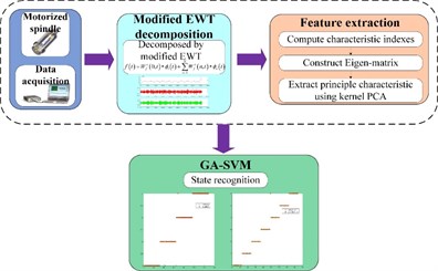
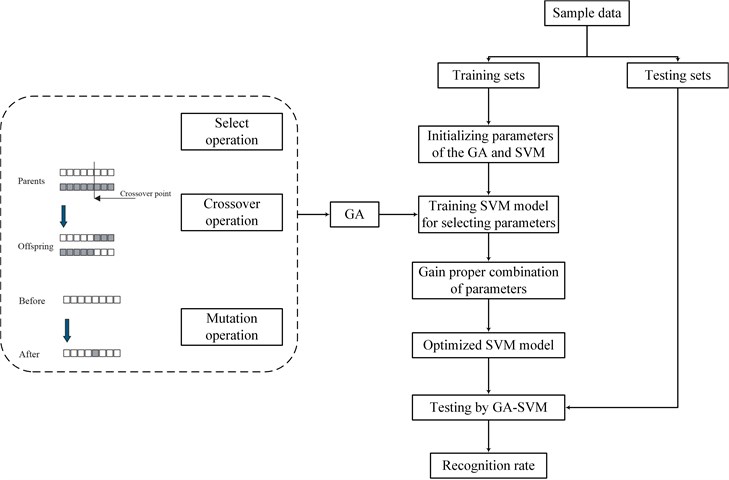
In this paper, a method combining modified EWT with Kernel PCA is applied in the single and compound fault diagnosis of the motorized spindle. Penalty wavelet threshold de-noising is adopted for data preprocessing before executing EWT, and a new approach is proposed to determine the number of the Fourier spectrum segment when using EWT. The SVM optimized by genetic algorithm (GA-SVM) is used as the multi-fault classifier because the SVM from statistical learning theory has better generalization property than conventional pattern recognition [48]. The performance of the proposed method is validated through single and compound fault experiments in a motorized spindle and is better compared with that of EMD, EEMD, LMD and EWT with proper number of segments. The flow chart of the present scheme is presented in Fig. 1.

Fig. 1Flow chart of the present scheme

The paper is arranged as follows: Section 2 briefly introduces the theoretical background of EWT, Kernel PCA, and SVM, and a new approach to decide the number of the Fourier spectrum segment when using EWT is also proposed. In Section 3, the data acquisition of single and compound faults in a motorized spindle is described in detail. Section 4 presents the data processing and experimental results. Moreover, a comparative study among modified EWT-Kernel PCA, EMD, EEMD, LMD and EWT (the proper number of segment is selected) is executed. Finally, conclusions are drawn in Section 5.

2. Methodology

2.1. Modified empirical wavelet transform

2.1.1. Empirical wavelet transform

EWT is a self –adaptive algorithm appropriate for processing non-linear and non-stationary signals by designing a series of bandpass filters. The self-adaptive property mainly embodies the support of filters depends on where the information embedded in the analyzed signal is situated. Signal modes are extracted by EWT, which are AM-FM components that have compact support to the Fourier spectrum [49]. Assuming that the Fourier spectrum $[0, π]$ (frequency $ω \in [0, π]$ ) is partitioned into $N$ consecutive segments, which correspond to different modes, $ω_{n}$ is defined as the limit between each segment (where $ω_{0} = 0$ and $ω_{n} = π$ ), and the transition phase, which exists centered around each $ω_{n}$ , is denoted as $T_{n}$ of width $2 τ_{n}$ . A proportional relationship between $ω_{n}$ and $τ_{n}$ exists, namely $ω_{n} : τ_{n} = γ ω_{n}$ , where $0 < γ < 1$ . The idea used in the construction of both Littlewood-Paley and Meyer’s wavelets is applied on the creation of empirical wavelets. For $\forall n > 0$ , the empirical scaling function ${\hat{ϕ}}_{n} (ω)$ and the empirical wavelets ${\hat{ψ}}_{n} (ω)$ are given by the following equations:

1

{\hat{ϕ}}_{n} (ω) = \{\begin{array}{l} 1, |ω| \leq (1 - γ) ω_{n}, \\ c o s [\frac{π}{2} β (\frac{1}{2 γ ω_{n}} (|ω|) - (1 - γ) ω_{n})], (1 - γ) ω_{n} \leq |ω| \leq (1 + γ) ω_{n} \\ 0, otherwise, \end{array},

2

{\hat{ψ}}_{n} (ω) = \{\begin{array}{l} 1, (1 + γ) ω_{n} \leq |ω| \leq (1 - γ) ω_{n + 1}, \\ c o s [\frac{π}{2} β (\frac{1}{2 γ ω_{n + 1}} (|ω| - (1 - γ) ω_{n + 1}))], (1 - γ) ω_{n + 1} \leq |ω| \leq (1 + γ) ω_{n + 1}, \\ s i n [\frac{π}{2} β (\frac{1}{2 γ ω_{n}} (|ω| - (1 - γ) ω_{n}))], (1 - γ) ω_{n} \leq |ω| \leq (1 + γ) ω_{n}, \\ 0, otherwise . \end{array}

To obtain a tight frame, parameter $γ$ satisfies following condition:

3

γ < m i n_{n} (\frac{ω_{n + 1} - ω_{n}}{ω_{n + 1} + ω_{n}}) .

The function $β (x)$ is an arbitrary $C^{k} ([0,1])$ function, such that:

4

β (x) = \{\begin{array}{l} 0, x \leq 0, β (x) + β (x + 1) = 1, \forall x \in [0,1], \\ 1, x \geq 1 . \end{array}

Numerous functions satisfy these properties, and the following function is frequently used [50]:

5

β (x) = x^{4} (35 - 84 x + 70 x^{2} - 20 x^{3}) .

Similar to wavelet transform, EWT is denoted as $W_{f}^{ε} (n, t)$ . Its detail coefficients are defined by the inner products of raw signals and the empirical wavelets, shown in the following equation:

6

W_{f}^{ε} (n, t) = \int f (τ) \bar{ψ_{n} (τ - t)} d τ .

The approximation coefficients are acquired by the inner products of raw signals and the scaling function as in the following equation:

7

W_{f}^{ε} (0, t) = \int f (τ) \bar{ϕ_{1} (τ - t)} d τ .

The reconstruction and the empirical mode $f_{k}$ are obtained by:

8

f (t) = W_{f}^{ε} (0, t) * ϕ_{1} (t) + \sum_{n = 1}^{N} W_{f}^{ε} (n, t) * ϕ_{n} (t),

9

\{\begin{array}{l} f_{0} (t) = W_{f}^{ε} (0, t) * ϕ_{1} (t), \\ f_{k} (t) = W_{f}^{ε} (k, t) * ψ_{k} (t), \end{array}

where $f$ is the signal, $t$ is the time, and $τ$ is the time variable.

2.1.2. Determine the number of the Fourier spectrum segment

In order to find the limits $ω_{n}$ between each segment, the method that computes the local maxima and then the boundaries are set as the smallest minima between consecutive maxima is adopted in this paper. However, the number of segments of the Fourier spectrum is difficult to determine because of lacking priori information for practical analysis. Excessive or less segment contradicts the effect of fault diagnosis. Therefore, determining the proper number of segments is crucial.

Fig. 2Framework of the proposed method

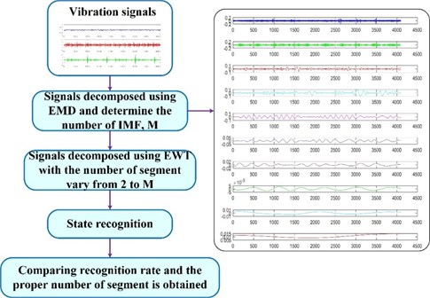
EMD is well known in suffering from mode mixing. The proper number of the Fourier spectrum segment is believed to be less than the number of IMF using EMD in this paper, and the IMF number is denoted as $M$ . Afterwards, the proper number of segments is easily determined by comparing the recognition rate of the fault diagnosis using GA-SVM with the number of segment vary from 2 to $M$ . The framework of the proposed method for determining the optimal number of EWT segments is shown in Fig. 2.

2.2. Kernel principal component analysis (Kernel PCA)

Although PCA can perform well in processing a set of linear data, it is not applicable for non-linear data. To deal with non-linear data, the extended version of PCA, KPCA, is introduced [51]. By using the kernel method, the non-linear data can be mapped into a higher dimensional space in which they vary linearly. Given a set of centered data $x_{k}$ , $k = 1, . . ., M$ , $x_{k} \in R^{d}$ , then these centered data are mapped into a higher dimensional feature space $F$ by non-linear mapping $ϕ : R^{d} \to F$ . Covariance matrix is computed in $F$ as:

10

\bar{C} = \frac{1}{M} \sum_{j = 1}^{M} ϕ (x_{j}) ϕ {(x_{j})}^{T} .

The eigenvalues $λ \geq 0$ and eigenvectors $V$ satisfy the following equation:

11

λ V = \bar{C} V = \frac{1}{M} \sum_{j = 1}^{M} (ϕ (x_{j}) \cdot V) ϕ (x_{j}) .

All solutions $V$ with $λ \neq 0$ lie in the span of $ϕ (x_{1}), . . . ϕ (x_{M})$ . Hence, the following equation is obtained:

12

\{\begin{array}{l} λ (ϕ (x_{k}) \cdot V) = (ϕ (x_{k}) \cdot \bar{C} V), k = 1, . . ., M, \\ V = \sum_{i = 1}^{M} α_{i} ϕ (x_{i}), \end{array}

where $α_{i} (i = 1, . . ., M)$ is the coefficient. According to Eq. (12), we can obtain:

13

λ \sum_{i = 1}^{M} α_{i} (ϕ (x_{k}) \cdot ϕ (x_{i})) = \frac{1}{M} \sum_{i = 1}^{M} α_{i} (ϕ (x_{k}) \cdot \sum_{j = 1}^{M} ϕ (x_{j})) (ϕ (x_{j}) \cdot ϕ (x_{i})) .

The kernel trick $K_{i j} = (ϕ (x_{i}) \cdot ϕ (x_{j}))$ is applied, and $K$ is the $M \times M$ kernel matrix. We can obtain:

14

M λ K α = K^{2} α,

where $α$ is the column vector with entries $α_{1}, . . ., α_{M}$ . To find the solutions of Eq. (14), we solve the eigenvalue problem:

15

M λ α = K α .

Define $λ_{1} \leq λ_{2} \leq \dots \leq λ_{M}$ as the eigenvalues of $K$ , $α^{1}, . . ., α^{M}$ , which are the corresponding complete set of eigenvectors, and $λ_{p}$ is the first non-zero eigenvalue. According to a specific requirement, normalization processing in feature space $F$ is executed for the corresponding eigenvectors $α^{1}, . . ., α^{M}$ where:

16

(V^{k} \cdot V^{k}) = 1, k = p, . . ., M .

By synthesizing Eq. (12) and Eq. (15), the following equation is obtained:

17

1 = \sum_{i, j = 1}^{M} α_{i}^{k} α_{j}^{k} (ϕ (x_{i}) \cdot ϕ (x_{j})) = \sum_{i, j = 1}^{M} α_{i}^{k} α_{j}^{k} K_{i j} = λ_{k} (α^{k} \cdot α^{k}) .

Computation of the projections onto the eigenvectors $V^{k}$ in $F$ is necessary to extract the principal component:

18

(V^{k} \cdot ϕ (x)) = \sum_{i = 1}^{M} α_{i}^{k} (ϕ (x_{i}) \cdot ϕ (x)) .

In addition, the problem on selecting the proper number of principal components has attracted considerable interests for the past decade. A series of criteria have been adopted in the selection of the number of principal components, and the most frequently used approach, that is, cumulative contribution limit [52], is applied in this paper.

2.3. Support vector machine optimized by genetic algorithm

SVM was first proposed by Vapnik et al. based on statistical learning theory [48]. Through time, SVM become increasingly popular in machine learning, and has been widely used in machine fault diagnosis because of its better generalization and higher recognition rate for analysis of small set of samples compared to traditional pattern recognition approaches such as artificial neural networks (ANN). The basic principle of SVM for typical two-class classification problems is described as follows. Given a set of training data $\{x_{i}, y_{i}\}$ , $1 \leq i \leq Q$ and $y_{i} \in \{- 1, + 1\}$ , SVM aims to find a high dimensional space in which the training data can be separated by the hyperplane as accurately as possible. In the linear separable case, the hyperplane can be expressed in the following equation:

19

w \cdot x + b = 0,

where $w$ is the $Q$ -dimensional vector, $x$ is the input vector, and $b$ is the scalar.

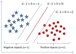
The training data are classified into two portions, and they are referred as negative and positive objects by hyperplane. The positive and negative object labels are $y_{i} = + 1$ and $y_{i} = - 1$ , respectively. An optimal separating hyperplane, which creates the maximum distance between two edge lines, depended on support vectors. A linear classification is shown in Fig. 3. The slack variables $ζ_{i}$ and the penalty parameter $C$ are introduced because of considering the noise. Thus, the optimal problem can be expressed as:

20

\begin{array}{l} minimize \frac{1}{2} {‖w‖}^{2} + C \sum_{i = 1}^{N} ζ_{i}, \\ subject to \{\begin{array}{l} y_{i} (w^{T} x_{i} + b) \geq 1 - ζ_{i}, \\ ζ_{i} \geq 0, i = 1, . . ., Q, \\ C \geq 0, \end{array} \end{array}

where $‖w‖$ is the Euclidean norm of $w$ .

Kernel transform is applied when the original data should be mapped into a higher feature space facing the non-linear problem, and $K$ is the kernel function. The SVM classifier output is then expressed as:

21

f (x) = s i g n (\sum_{i = 1}^{N} μ_{i} y_{i} K (x, x_{i}) + b),

where $μ_{i}$ is the Lagrange multipliers and $x_{i}$ is the support vector.

Fig. 3Linear classification

Radial basis function is a common kernel function, and it has been used as kernel of SVM in numerous articles. Hence, it is chosen as the kernel function in this study. The radial basis function is defined as follows:

22

K (x, x_{i}) = e x p (- γ {‖x - x_{i}‖}^{2}) .

In which $γ = 1 / 2 σ^{2}$ is the kernel parameter and $σ$ is the width parameter of the radical basis function.

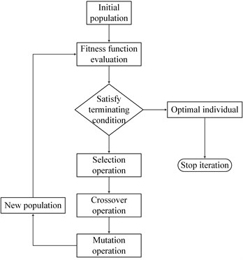
It is essential to select a proper combination of parameters for achieving best prediction accuracy in SVM. It is well known that the GA is a global optimization algorithm based on Charles Darwin’s theory of natural selection and evolution, and it is a powerful tool to solve the optimization problem. Therefore, in order to find the best parameter combination, the GA [53] is applied into SVM. The steps of a simple GA are shown in Fig. 4. In this paper, population size, the number of iterations, crossover probability and mutation probability are set to 20, 200, 0.9 and 0.05, respectively. GA is introduced to find a proper combination of parameters, namely $C$ and $γ$ , and the value ranges are both set to the range of 0 to 200. In addition, the SVM recognition rate serves as the fitness function. The flowchart of GA-SVM is presented in Fig. 5.

Fig. 4Genetic algorithm flowchart

3. Data acquisition of single and compound faults

According to the statistical analysis, bearing fault contributes the largest proportion, accounting for 44.4 %, in the mechanical spindle of machining center [54]. Thus, execution of bearing fault diagnosis of the motorized spindle is necessary. In addition, rotor unbalance and bolt looseness fault immensely impact the performance of motorized spindle. To verify the effectiveness of the proposed method, the bearing fault data, which comes from the bearing data center of Case Western Reserve University was utilized for single fault diagnosis [55]. As for the compound fault diagnosis, vibration data was acquired in different fault conditions, namely normal, rotor unbalance, bolt looseness, and compound fault (rotor unbalance and bolt looseness coexist).

Fig. 5Flowchart for GA-SVM

3.1. Data acquisition of single faults

Experiments for bearing single faults were conducted in a test stand. The test stand is composed of a three-phase induction motor, an AC electrical dynamometer, a torque sensor, and a control system. The 6205-2RS JEM SKF, deep groove ball bearing, was selected as test bearing, which supports the induction motor shaft. The localized defects were created on the inner and outer raceways and the ball by utilizing electro-discharge machining. The diameters of single point faults were 0.1778 and 0.3556 mm, and the depth of defect was consistent at 0.2794 mm. Accelerometers were used to acquire vibration signals, which were fixed in the drive end of the induction motor housing with magnetic bases, in which the laying position was at the 6 o’clock position. The vibration signals were acquired at a sampling frequency of 12000 Hz, and the motor output speed was 1772 rpm with 1 horsepower motor load.

3.2. Data acquisition of compound faults

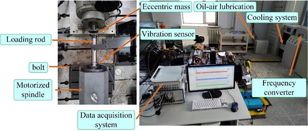
Compound fault experiments in a motorized spindle were conducted in the test platform as shown in Fig. 6.

The test platform consists of a data acquisition system, oil-air lubrication, cooling system, frequency converter, loading rod, and a motorized spindle. The loading rod was installed in the motorized spindle, and the eccentric mass was fixed in the loading rod, which realizes the fault simulation for rotor unbalance. In addition, the motorized spindle was fixed by four bolts, and three of them were loosened when the bolt looseness fault experiment was conducted. Considering safety, the speed of the motorized spindle was set to 5000 rpm. Vibration signals were collected in various states at a sampling frequency of 5000 Hz. Electromagnetic interference should be given attention because of the frequency converter. Therefore, vibration signals were preprocessed using Penalty wavelet threshold de-noising, which can increase SNR.

Fig. 6Test platform of the motorized spindle

4. Data processing and experimental results

4.1. Single fault diagnosis

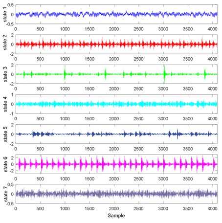
In the experiment of single faults, vibration signals are collected in seven states, namely the normal condition, the inner raceway fault (two states with different fault diameters), the ball fault (two states with different fault diameters), and the outer raceway fault (two states with different fault diameters). The fault diameters are 0.1778 mm and 0.3556 mm respectively. The time domain waveforms of vibration signals collected in seven states are presented in Fig. 7. Single fault diagnosis aims to identify the seven states effectively and accurately. Vibration signals collected in a certain state are divided into 29 subsets with equal lengths of 4096. A detailed description for vibration signals is shown in Table 1.

Fig. 7Time domain waveforms of vibration signals

The EWT-Kernel PCA method is applied to process vibration signals. To start with, the proper number of segment needs to be determined. EMD is initially applied to analyze vibration signals, and the number of intrinsic mode function obtained using EMD is between 10 and 12. Considering that EMD suffers from the major shortcoming of mode mixing, the determination of the proper number of segment is reasonably not larger than 10. Vibration signals collected at different states are then decomposed using EWT, and the number of segment varies from 2 to 10. Energy, kurtosis, and root mean square are selected as characteristic indexes. Characteristic indexes of the signals, which are decomposed by using EWT, are extracted to construct Eigen-matrix which serves as input of GA-SVM. The recognition rate is obtained using GA-SVM, and the results are presented in Table 2. The proper number of segment is determined by comparing the recognition rate.

Table 1Detailed description of vibration signals

Class	Bearing fault	Defect size (mm)	Sample number
State 1	Normal	0	29
State 2	Inner raceway	0.1778	29
State 3	Inner raceway	0.3556	29
State 4	Ball	0.1778	29
State 5	Ball	0.3556	29
State 6	Outer raceway	0.1778	29
State 7	Outer raceway	0.3556	29

Table 2Recognition rate (single faults)

Number of segment	Recognition rate (%)	Time (s)
2	98.8095	24.0550
3	100	25.9561
4	97.6190	26.9161
5	95.2381	27.7974
6	95.2381	32.0490
7	95.2381	32.1671
8	96.4286	32.5506
9	94.0476	33.2683
10	94.0476	33.7320

According to Table 2, the highest recognition rate is easily found when the number of segment varies from 2 to 10. From Table 2, we can see that the highest recognition rate is 100 % when the number of segment is 3; therefore, the proper number of segment is 3. Kernel PCA is applied to extract the principal characteristics from Eigen-matrix. Furthermore, cumulative contribution limit is adopted to determine the number of principal characteristics. The detailed description for cumulative contribution is presented in Table 3.

Table 3Cumulative contribution

Serial number	Eigenvalue	Cumulative contribution
1	124.6073	0.6412
2	24.2019	0.7657
3	16.1617	0.8489
4	9.6115	0.8984
5	7.7455	0.9382
6	4.9167	0.9635
7	3.0010	0.9790
8	2.6911	0.9928
9	1.3953	1

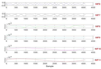
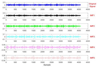
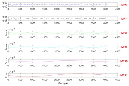
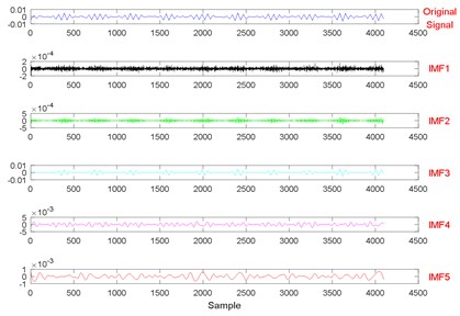
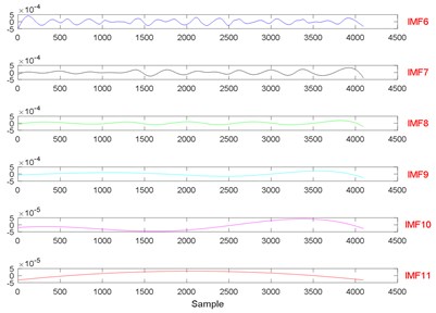
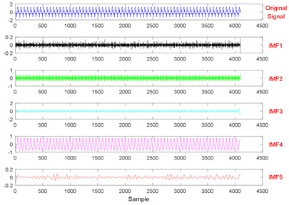
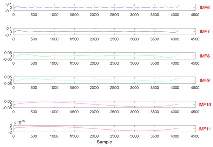
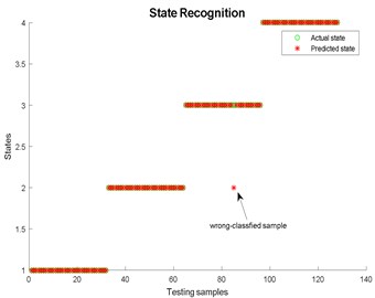
The threshold of cumulative contribution limit is set to 0.90 in this paper. According to Table 3, the anterior five characteristics are extracted as principal characteristics. Finally, the new Eigen-matrix serves as the input of GA-SVM. Table 1 shows that a total of 29 samples are obtained in each state, and the anterior 60 % of samples are selected as training samples. For comparison, EMD, EEMD and LMD are applied to decompose vibration signals collected in different states as well. When using EEMD, there are two parameters are needed to be set, which are the ensemble number and the amplitude of the added white noise. In this study, the ensemble number and the amplitude of the added white noise are set to 100 and 0.2, respectively [56]. The results of EEMD/EWT/LMD decomposition are given in Figs. 8-13. In this paper, we only give the results of two states, namely State 1 (Normal) and State 7 (Outer raceway fault, the defect size is 0.3556 mm) because of limited space. Then energy, kurtosis, and root mean square are computed to construct an Eigen-matrix, which is inputted in GA-SVM, and the result is shown in Figs. 14-17. A detailed comparison results for single fault diagnosis is presented in Table 4. According to Table 4, modified EWT-Kernel PCA, EWT ( $N =$ 3), EEMD and LMD are superior to EMD in two aspects: recognition rate and computing time. In addition, modified EWT–Kernel PCA, EWT ( $N =$ 3), EEMD and LMD can reach a high recognition rate. As for computing time, the modified EWT-Kernel PCA is better than EWT ( $N =$ 3), EEMD and LMD.

Fig. 8The signal decomposition of State 1 by EEMD

a)

b)

Fig. 9The signal decomposition of State 7 by EEMD

a)

b)

Fig. 10The signal decomposition of State 1 by EWT

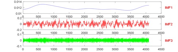
Fig. 11The signal decomposition of State 7 by EWT

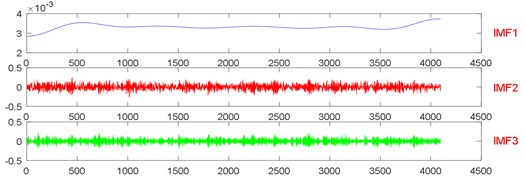
Fig. 12The signal decomposition of State 1 by LMD

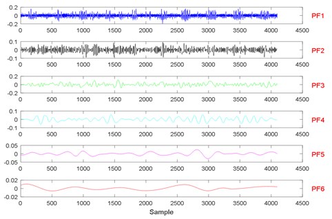
Fig. 13The signal decomposition of State 7 by LMD

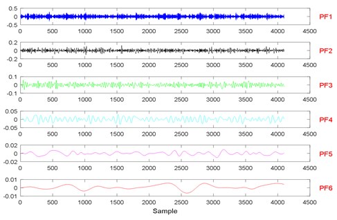
Fig. 14State recognition using the modified EWT-Kernel PCA

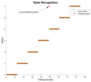
Fig. 15State recognition using EMD

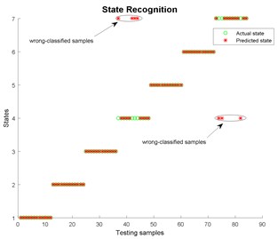
Fig. 16State recognition using EEMD

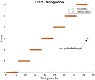
Fig. 17State recognition using LMD

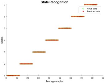
Table 4Comparison results (single fault diagnosis)

Method	Recognition rate (%)	Time (s)	Optimum parameters
Method	Recognition rate (%)	Time (s)	$C$	$γ$
Modified EWT-Kernel PCA	98.8095	20.8028	2.9676	18.6115
EWT ( $N =$ 3)	100	25.9561	21.5076	1.9846
EMD	91.6667	32.4293	3.2776	0.7719
EEMD	98.8095	27.3467	13.4472	0.4829
LMD	100	27.9825	6.8211	1.0040

4.2. Compound fault diagnosis

In the compound fault experiment, vibration signals are collected in four states, namely normal, rotor unbalance, bolt looseness, and compound fault (rotor unbalance and bolt looseness coexist). The time domain waveforms of vibration signals, which are preprocessed using Penalty wavelet threshold de-noising, are presented in Fig. 18.

To identify the four states effectively and accurately, the preprocessed vibration signals are segmented into 80 subsets of equal lengths of 4096. Further description is presented in Table 5.

Fig. 18Time domain waveform of vibration signals

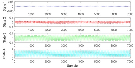
Table 5Further description of the preprocessed vibration signals

Class	Fault	Sample number
State 1	Normal	80
State 2	Bolt looseness	80
State 3	Rotor unbalance	80
State 4	Compound fault	80

The processing procedures of compound fault diagnosis are the same as that of single fault diagnosis. EMD is initially utilized to analyze vibration signals, and the number of intrinsic mode function obtained using EMD is between 9 and 11. The proper number of segment is considered less than 9 because EMD suffers from mode mixing. Vibration signals collected in four states are then decomposed using EWT, and the number of segment varies from 2 to 9. Energy, kurtosis and root mean square are extracted to construct Eigen-matrix, which serves as the input of GA-SVM. The results are presented in Table 6. The comparison results of the recognition rates of compound fault diagnosis revealed that the proper number of segment can be found.

Table 6Recognition rate (compound faults)

Number of segment	Recognition rate (%)	Time (s)
2	49.2188	24.6227
3	75.7813	26.6460
4	88.2813	26.4702
5	97.6563	25.1563
6	78.1250	27.3122
7	95.3125	24.1459
8	96.0938	26.7265
9	81.2500	28.1158

Table 6 shows that the highest recognition rate is obtained when the number of segment varies from 2 to 9. Hence, the proper number of segment is 5. Kernel PCA is applied to extract principal characteristics from Eigen-matrix. Cumulative contribution limit is adopted to determine the number of principal characteristics. The detailed description for cumulative contribution is presented in Table 7.

Table 7Cumulative contribution

Serial number	Eigenvalue	Cumulative contribution
1	119.2375	0.5610
2	14.9248	0.6312
3	14.0555	0.6973
4	11.8911	0.7533
5	9.2964	0.7970
6	7.0838	0.8303
7	6.5162	0.8610
8	5.6663	0.8877
9	4.9138	0.9108
10	4.3771	0.9314
11	3.9011	0.9497
12	2.9933	0.9638
13	2.7913	0.9769
14	2.5411	0.9889
15	2.3607	1

According to Table 7, because the threshold of the cumulative contribution limit is set to 0.90 in this paper, the anterior nine characteristics are extracted as principal characteristics. Finally, the new Eigen-matrix serves as the input of GA-SVM. Based on Table 5, a total of 80 samples are obtained in each state, and the anterior 60 % of samples are selected as training samples. The results of EEMD/EWT/LMD decomposition are given in Figs. 19-24. In this paper, we only give the results of two states, namely State 1 (Normal) and State 4 (Compound fault) because of limited space. The results of state recognition using modified EWT-Kernel PCA, EMD, EEMD and LMD are shown in Figs. 25-28. The result of the detailed comparison of compound fault diagnosis is presented in Table 8. According to Table 8, modified EWT-Kernel PCA, EWT ( $N =$ 5) EEMD and LMD are obviously far superior to EMD in terms of recognition rate. For computing time, the modified EWT-Kernel PCA is better than EWT ( $N =$ 5), EMD, EEMD and LMD.

Table 8Comparison results (compound faults diagnosis)

Method	Recognition rate (%)	Time (s)	Optimum parameters
Method	Recognition rate (%)	Time (s)	$C$	$γ$
Modified EWT-Kernel PCA	98.4375	18.0463	104.7613	1.5739
EWT ( $N =$ 5)	97.6563	25.1563	87.7794	1.8892
EMD	94.5313	43.0471	46.9961	0.9804
EEMD	99.2188	43.5325	100.1085	0.8619
LMD	99.2188	20.2320	9.3590	0.5783

Fig. 19The signal decomposition of State 1 by EEMD

a)

b)

Fig. 20The signal decomposition of State 4 by EEMD

a)

b)

Fig. 21The signal decomposition of State 1 by EWT

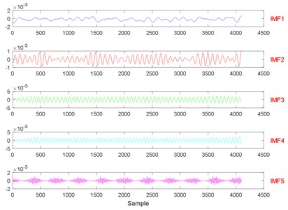
Fig. 22The signal decomposition of State 4 by EWT

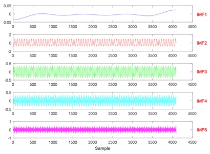
Fig. 23The signal decomposition of State 1 by LMD

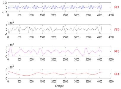
Fig. 24The signal decomposition of State 4 by LMD

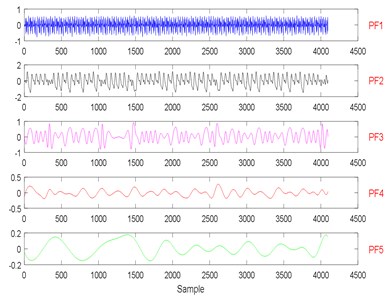
Fig. 25State recognition using modified EWT-Kernel PCA

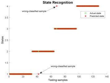
Fig. 26State recognition using EMD

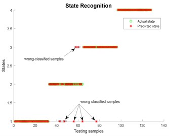
Fig. 27State recognition using EEMD

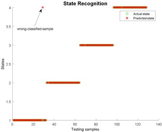
Fig. 28State recognition using LMD

5. Conclusions

In this paper, a method based on modified EWT and Kernel PCA for the single and compound fault diagnoses of the motorized spindle is investigated. A comparison study among EWT (the proper number of segment is selected), EMD, EEMD, LMD and modified EWT-Kernel PCA is executed. The experimental data obtained from the bearing data center of Case Western Reserve University are utilized for the single fault diagnosis of a motorized spindle, and as for compound fault diagnosis, experiments are carried out on a test platform for a motorized spindle. The analysis results indicate that the proposed method can effectively and correctly performs fault diagnosis. The recognition rate using modified EWT-Kernel PCA reach 98.8095 % and 98.4375 % in terms of single and compound fault diagnoses, respectively, which are higher than those in EMD. Moreover, for single fault diagnosis, the recognition rate using modified EWT-Kernel PCA, EWT, EEMD and LMD are almost the same, and as for compound fault diagnosis, modified EWT-Kernel PCA, EEMD and LMD are superior to EWT ( $N =$ 5) and EMD. Compared with EWT, EMD, EEMD and LMD in the aspect of computing time, the proposed method saved 19 %, 35 %, 24 % and 26 % for single fault diagnosis, respectively. For compound fault diagnosis, the proposed method saved 39 %, 58 %, 59 % and 11 %, respectively. Finally, this method can be generalized for another mechanical fault diagnosis.

References

Bossmanns B., Tu J. F. A thermal model for high speed motorized spindles. International Journal of Machine Tools and Manufacture, Vol. 39, Issue 9, 1999, p. 1345-1366.

Publisher
Wu Y. H. Motorized Spindle Unit Technology of CNC Machine Tools. China Machine Press, Beijing, 2006.

Search CrossRef
Abele E., Altintas Y., Brecher C. Machine tool spindle units. CIRP Annals – Manufacturing Technology, Vol. 59, Issue 2, 2010, p. 781-802.

Publisher
Shan W. T., Chen X. A., He Y., Zhou J. M. A novel experimental research on vibration characteristics of the running high-speed motorized spindles. Journal of Mechanical Science and Technology, Vol. 27, Issue 8, 2013, p. 2245-2252.

Publisher
Liu J. F., Chen X. A. Dynamic design for motorized spindles based on an integrated model. The International Journal of Advanced Manufacturing Technology, Vol. 71, Issue 9, 2014, p. 1961-1974.

Publisher
Marquez F. P. G., Tobias A. M., Perez J. M. P., Papaelias M. Condition monitoring of wind turbines: techniques and methods. Renew Energy, Vol. 46, 2012, p. 169-178.

Publisher
Yang W. X., Little C., Court R. An online technique for condition monitoring the induction generators used in wind and marine turbines. Mechanical Systems and Signal Processing, Vol. 38, Issue 1, 2013, p. 103-112.

Publisher
Yang W. X., Little C., Court R. S-Transform and its contribution to wind turbine condition monitoring. Renew Energy, Vol. 62, 2014, p. 137-146.

Publisher
Cao H. R., Fan F., Zhou K., He Z. J. Wheel-bearing fault diagnosis of trains using empirical wavelet transform. Measurement, Vol. 82, 2016, p. 439-449.

Publisher
Amezquita-Sanchez J. P., Adeli H. A new music-empirical wavelet transform methodology for time-frequency analysis of noisy nonlinear and non-stationary signals. Digital Signal Process, Vol. 45, 2015, p. 55-68.

Search CrossRef
Allen J. B. Short term spectral analysis, synthesis, and modification by discrete Fourier transform. IEEE Transactions on Acoustics, Speech, and Signal Processing, Vol. 25, Issue 3, 1977, p. 235-238.

Publisher
Baydar N., Ball Andrew A comparative study of acoustic and vibration signals in detection of gear failures using Wigner-Ville distribution. Mechanical Systems and Signal Process, Vol. 15, Issue 6, 2001, p. 1091-1107.

Publisher
Peng Z. K., Chu F. L. Application of the wavelet transform in machine condition monitoring and fault diagnostics: a review with bibliography. Mechanical Systems and Signal Process, Vol. 18, Issue 2, 2004, p. 199-221.

Publisher
Yu B., Jia L., Ji C., Lin S., Yun L. Trains trouble shooting based on wavelet analysis and joint selection feature classifier. Journal of Multimedia, Vol. 9, Issue 2, 2014, p. 207-215.

Publisher
Mehala N., Dahiya R. A Comparative study of FFT, STFT and wavelet techniques for induction machine fault diagnostic analysis. Proceedings of the 7th Wseas International Conference on Computational Intelligence, Man-Machine Systems and Cybernetics, 2008, p. 203-208.

Search CrossRef
Valtierra-Rodriguez M., Romero-Troncoso R. J., Osornio-Rios R. A., Garcia-Perez A. Detection and classification of single and combined power quality disturbances using neural networks. IEEE Transactions on Industrial Electronics, Vol. 61, Issue 5, 2013, p. 2473-2482.

Publisher
Mallat S. G. A Wavelet Tour of Signal Processing: The Sparse Way. Elsevier/Academic Press, Amsterdam, 2009.

Search CrossRef
Zhang Y. Signals’ Time-Frequency Analysis and Its Application. Harbin Institute of Technology Press, Harbin, 2006.

Search CrossRef
Xiang L., Tang G. J., Hu A. J. Vibration signals’ time-frequency analysis and comparison for a rotating machinery. Journal of Vibration and shock, Vol. 29, Issue 2, 2010, p. 42-45.

Search CrossRef
Spanos P. D. A., Giaralis N., Politis P. Time-frequency representation of earthquake accelerograms and inelastic structural response records using the adaptive chirplet decomposition and empirical mode decomposition. Soil Dynamics and Earthquake Engineering, Vol. 27, Issue 7, 2007, p. 675-689.

Publisher
Li Z., He Z. J., Zi Y. Y., Wang Y. Customized wavelet denoising using intra-and inter-scale dependency for bearing fault detection. Journal of Sound and Vibration, Vol. 313, Issues 1-2, 2008, p. 342-359.

Publisher
Sun H. L., Zi Y. Y., He Z. J., Yuan J., Wang X. D., Chen L. Customized multiwavelets for planetary gearbox fault detection based on vibration sensor signals. Sensor, Vol. 13, Issue 1, 2013, p. 1183-1209.

Publisher
Ebrahimi B. M., Faiz J., Lotfi-Fard S., Pillay P. Novel indices for broken rotor bars fault diagnosis in induction motors using wavelet transform. Mechanical Systems and Signal Processing, Vol. 30, 2012, p. 131-145.

Publisher
Yan R. Q., Gao R. X., Chen X. F. Wavelets for fault diagnosis of rotary machines: a review with applications. Signal Processing, Vol. 96, 2014, p. 1-15.

Publisher
Djebala A., Ouelaa N., Hamzaoui N. Detection of rolling bearing defects using discrete wavelet analysis. Meccanica, Vol. 43, Issue 3, 2008, p. 339-348.

Publisher
Lei Y. G., Lin J., He Z. J., Zuo M. J. A review on empirical mode decomposition in fault diagnosis of rotating machinery. Mechanical Systems and Signal Processing, Vol. 35, Issues 1-2, 2013, p. 108-126.

Publisher
Yeh P. L., Liu P. L. Application of the wavelet transform and the enhanced Fourier spectrum in the impact echo test. NDT&E International, Vol. 41, Issue 5, 2008, p. 382-394.

Publisher
Huang N. E., Shen Z., Long S. R. The empirical mode decomposition and the Hilbert spectrum for nonlinear and non-stationary time series analysis. Proceedings of Mathematical, Physical and Engineering Sciences, Vol. 454, Issue 1971, 1998, p. 1294-1306.

Publisher
Kedadouche M., Thomas M., Tahan A. Empirical mode decomposition of acoustic emission for early detection of bearing defects. Proceedings of the 3rd International Conference on Condition Monitoring of Machinery in Non-Stationary Operations (CMMNO), 2013, p. 367-377.

Publisher
Qin Y. Multicomponent AM-FM demodulation based on energy separation and adaptive filtering. Mechanical Systems and Signal Processing, Vol. 38, Issue 2, 2013, p. 440-459.

Publisher
Wu Z., Huang N. Ensemble empirical mode decomposition: a noise-assisted data analysis method. Advances in Adaptive Data Analysis, Vol. 1, Issue 1, 2009, p. 1-41.

Search CrossRef
Loh C. H., Wu T. C., Huang N. E. Application of the empirical mode decomposition Hilbert spectrum method to identify near-fault ground-motion characteristics and structural responses. Seismological Society of America, Vol. 91, Issue 5, 2001, p. 1339-1357.

Publisher
Meng Z., Gu H. Y., Li S. S. Restraining method for end effect of B-spine empirical mode decomposition based on neural network ensemble. Journal of Mechanical Engineering, Vol. 49, Issue 9, 2013, p. 106-112.

Publisher
Wu Z. H., Huang N. E. Ensemble empirical mode decomposition: a noise-assisted data analysis method. Advances in Adaptive Data Analysis, Vol. 1, Issue 1, 2009, p. 1-41.

Publisher
Lei Y. G., He Z. J., Zi Y. Y. Application of the EEMD method to rotor fault diagnosis of rotating machinery. Mechanical Systems and Signal Processing, Vol. 23, Issue 4, 2009, p. 1327-1338.

Publisher
Bin G. F., Gao J. J., Li X. J., Dhillon B. S. Early fault diagnosis of rotating machinery based on wavelet packets – empirical mode decomposition feature extraction and neural network. Mechanical Systems and Signal Processing, Vol. 27, 2012, p. 696-711.

Publisher
Widodo A., Yang B. S., Han T. Combination of independent component analysis and support vector machines for intelligent faults diagnosis of induction motors. Expert Systems with Applications, Vol. 32, Issue 2, 2007, p. 299-312.

Publisher
Zvokelj M., Zupan S., Prebi I. Multivariate and multiscale monitoring of large-size low-speed bearings using ensemble empirical mode decomposition method combined with principal component analysis. Mechanical Systems and Signal Processing, Vol. 24, Issue 4, 2010, p. 1049-1067.

Publisher
Han M. H., Pan J. L. A fault diagnosis method combined with LMD, sample entropy and energy ratio for roller bearings. Measurement, Vol. 76, 2015, p. 7-19.

Publisher
Du Y. P., Zhang W. J., Zhang Y., Gao Z. Q., Wang X. H. Fault diagnosis of rotating machines for rail vehicles based on local mean decomposition-energy moment-directed acyclic graph support vector machine. Advances in Mechanical Engineering, Vol. 8, Issue 1, 2016, p. 1-6.

Publisher
Liua B., Riemenschneider S., Xu Y. Gearbox fault diagnosis using empirical mode decomposition and Hilbert spectrum. Mechanical Systems and Signal Processing, Vol. 20, Issue 3, 2006, p. 718-734.

Publisher
Gilles J. Empirical wavelet transform. IEEE Transactions on Signal Processing, Vol. 61, Issue 16, 2013, p. 3999-4010.

Publisher
Xu T. L., Zhang X. Y., Jia Q. X., Lang X. Z. Rolling bearing fault research on wavelet threshold de-noising. Journal of Ship Mechanics, Vol. 16, Issue 10, 2012, p. 1199-1203.

Search CrossRef
Shuai J. N. Research on Acoustic Emission Signals for the Damage of the Fan Blade Based on De-Noising Technology and Blind Source. Nanjing University of Aeronautics and Astronautics, No. 1028701 14-S114, 2013.

Search CrossRef
Kedadouche M., Liu Z. H., Vu V. H. A new approach based on OMA-empirical wavelet transforms for bearing fault diagnosis. Measurement, Vol. 90, 2016, p. 292-308.

Publisher
Juan P., Sanchez A., Adeli H. A new music-empirical wavelet transform methodology for time-frequency analysis of noisy non-linear and non-stationary signals. Digital Signal Processing, Vol. 45, 2015, p. 55-68.

Publisher
Caoa L. J., Chuab K. S., Chong W. K., Lee H. P., Gu Q. M. A comparison of PCA, KPCA and ICA for dimensionality reduction in support vector machine. Neurocomputing, Vol. 55, 2003, p. 321-336.

Publisher
Vapnik V. N. The Nature of Statistical Learning Theory. Springer, New York, 1995.

Publisher
Daubechies I., Lu J. F., Wu H. T. Synchrosqueezed wavelet transforms: an empirical mode decomposition-like tool. Applied and Computational Harmonic Analysis, Vol. 30, Issue 2, 2011, p. 243-261.

Publisher
Daubechies I. Ten lectures on wavelets. The Journal of the Acoustical Society of America, Vol. 93, Issue 3, 1992, p. 1671.

Publisher
Bernhard S., Alexander S., Klaus-Robert M. Nonlinear component analysis as a kernel eigenvalue problem. Neural Computation, Vol. 10, Issue 5, 1998, p. 1299-1319.

Publisher
Li G. Z. Discussion on Selecting the Number of Principal Components. Lanzhou University of Finance and Economics, No. 10741, 2015.

Search CrossRef
Holland J. H. Adaptation in Natural and Artificial Systems: an Introductory Analysis with Applications to Biology, Control, and Artificial Intelligence. MIT Press, Cambridge, 1992.

Publisher
Yang C. G. Development of Condition Monitoring System of Motorized Spindle Based on LabVIEW. Jilin University, No. TG659, 2015.

Search CrossRef
Bearing Data Center Seeded Fault Test Data [EB/OL]. The Case Western Reserve University Bearing Data Center Website, 2007, http://csegroups.case.edu/bearingdatacenter/ pages/download-data-file.

Search CrossRef
Hou M. M. Determination of Trace Moisture in Oil by the Measurement of Near Infrared Spectroscopy. Chongqing Technology and Business University, 2012.

Search CrossRef

Cited by

Rolling Bearing Compound Fault Diagnosis Based on Parameter Optimization MCKD and Convolutional Neural Network

Shuzhi Gao | Shuo Shi | Yimin Zhang

(2022)

Research on singular spectrum decomposition and its application to rotor failure detection

Bin Pang | Guiji Tang | Yuling He

(2018)

About this article

Received

30 January 2017

Accepted

27 April 2017

Published

30 June 2017

SUBJECTS

Fault diagnosis based on vibration signal analysis

DOI

https://doi.org/10.21595/jve.2017.18214

Keywords

motorized spindle

fault diagnosis

modified empirical wavelet transform (EWT)

kernel principal components analysis (Kernel PCA)

Acknowledgements

This work is supported by the Project of Jilin Province, Science and Technology Development Plan of the Fault Diagnosis and Condition Monitoring for Motorized Spindle of Machining Center (Grant No. 20160101278JC) and the Subject of the Research and Application of Rapid Test Technology for Reliability of CNC (Grant No. 2016ZX04004-004) and the Project of the Graduate Innovation Fund of Jilin University (Grant No. 2016027).

Author Contributions

Fei Chen conceived the idea of using modified empirical wavelet transform to analyze vibration data. Chao Chen applied kernel principal component analysis into reducing dimension and guide the writing of the whole paper. Yifeng Ye conducted the method to better diagnosis the single and compound fault of the motorized spindle and wrote the majority of the paper. Weizheng Chen Carried out the experiments. Binbin Xu processed the experimental data and analyzed the results. Zhaojun Yang edited the manuscript and checked the grammatical and spelling errors.

This is an open access article distributed under the Creative Commons Attribution License, which permits unrestricted use, distribution, and reproduction in any medium, provided the original work is properly cited.

Previous article in issue Previous Next article in issue Next

Research article

2023 10 09

Extraction and diagnosis of rolling bearing fault signals based on improved wavelet transform

Zhiqing Cheng

Research article

2023 08 01

Motor rolling bearing fault diagnosis based on MVMD energy entropy and GWO-SVM

Jian Tang, Qiaoni Zhao

Research article

2022 05 15

The enhancement of fault detection for rolling bearing via optimized VMD and TQWT based sparse code shrinkage

Xing Yuan, Huijie Zhang, Hui Liu

Research article

2019 09 30

Bearing fault diagnosis based on feature extraction of empirical wavelet transform (EWT) and fuzzy logic system (FLS) under variable operating conditions

Fawzi Gougam, Chemseddine Rahmoune, Djamel Benazzouz, Boualem Merainani

F. Chen, Y. Ye, W. Chen, B. Xu, C. Chen, and Z. Yang, “Fault diagnosis of motorized spindle via modified empirical wavelet transform-kernel PCA and optimized support vector machine,” Journal of Vibroengineering, Vol. 19, No. 4, pp. 2611–2631, Jun. 2017, https://doi.org/10.21595/jve.2017.18214

Copy Extrica

Copied to clipboard!

TY  - JOUR
DO  - 10.21595/jve.2017.18214
UR  - https://doi.org/10.21595/jve.2017.18214
TI  - Fault diagnosis of motorized spindle via modified empirical wavelet transform-kernel PCA and optimized support vector machine
T2  - Journal of Vibroengineering
AU  - Chen, Chao
AU  - Chen, Fei
AU  - Ye, Yifeng
AU  - Chen, Weizheng
AU  - Xu, Binbin
AU  - Yang, Zhaojun
PY  - 2017
DA  - 2017/06/30
PB  - JVE International Ltd.
SP  - 2611-2631
IS  - 4
VL  - 19
SN  - 1392-8716
ER  - 

Copy Ris

Copied to clipboard!

@article{Chen_2017,
	doi = {10.21595/jve.2017.18214},
	url = {https://doi.org/10.21595/jve.2017.18214},
	year = 2017,
	month = {jun},
	publisher = {{JVE} International Ltd.},
	volume = {19},
	number = {4},
	pages = {2611--2631},
	author = {Chao Chen and Fei Chen and Yifeng Ye and Weizheng Chen and Binbin Xu and Zhaojun Yang},
	title = {Fault diagnosis of motorized spindle via modified empirical wavelet transform-kernel {PCA} and optimized support vector machine},
	journal = {Journal of Vibroengineering}
}

Copy Bibtex

Copied to clipboard!

[1]C. Chen, F. Chen, Y. Ye, W. Chen, B. Xu, and Z. Yang, “Fault diagnosis of motorized spindle via modified empirical wavelet transform-kernel PCA and optimized support vector machine,” Journal of Vibroengineering, vol. 19, no. 4, pp. 2611–2631, Jun. 2017, doi: 10.21595/jve.2017.18214.

Copy IEEE

Copied to clipboard!

Chen, Chao, Fei Chen, Yifeng Ye, Weizheng Chen, Binbin Xu, and Zhaojun Yang. “Fault Diagnosis of Motorized Spindle via Modified Empirical Wavelet Transform-Kernel PCA and Optimized Support Vector Machine.” Journal of Vibroengineering 19, no. 4 (June 30, 2017): 2611–31. https://doi.org/10.21595/jve.2017.18214.

Copy Chicago

Copied to clipboard!

Fault diagnosis of motorized spindle via modified empirical wavelet transform-kernel PCA and optimized support vector machine

Abstract

1. Introduction

2. Methodology

2.1. Modified empirical wavelet transform

2.1.1. Empirical wavelet transform

2.1.2. Determine the number of the Fourier spectrum segment

2.2. Kernel principal component analysis (Kernel PCA)

2.3. Support vector machine optimized by genetic algorithm

3. Data acquisition of single and compound faults

3.1. Data acquisition of single faults

3.2. Data acquisition of compound faults

4. Data processing and experimental results

4.1. Single fault diagnosis

4.2. Compound fault diagnosis

5. Conclusions

References

Cited by

About this article

Related Articles