On the detection of self-similarities in vibro-acoustic signals

1. Introduction

The constantly growing interest in the condition monitoring, i.e. in the data extracted from vibro-acoustic signature of a machinery (vibration, temperature, electrocardiography, etc.) [1], has encouraged a new outlook towards the information stored in databases. The storage of raw data is of little value and so there can be seen a strong need to develop methods allowing to index, classify and process extensive data flows coming from various fields.

Preliminary processing of all types of data is the first step to making data analysis easier, therefore the increased attention to queries related to real vibro-acoustic signals and to the organization of data mining, not surprisingly, has good reasons. Besides, data mining is a very broad field; quite a few methods, algorithms and applied systems have been developed for this reason [2, 3].

In the data acquisition area, one encounters problems of interpolation, forecasting, feature extraction, early fault diagnosis, exposing fractal nature and others, which are usually associated with fragmentary analysis of vibro-acoustic (and not only) signals. Fragmentary analysis of signals usually employs the brute force procedures which are heavily time-consuming. One of the possible ways to avoid this difficulty is to solve the so-called signal similarity problem by introducing various metrics [4, 5]. The solution leans upon the use of the necessary signal similarity condition [6-8]. Then fragmentary analysis of vibro-acoustic signals is replaced by comparing fragmentary smoothness parameter values attached to signal fragments under investigation. The appreciable speed gains are achieved, and the door for the real-time preliminary signal processing is opened.

This paper introduces the context where the problem on the detection of similar fragments in the vibro-acoustic signals is formulated and solved.

2. The notion of fragmentary smoothness of vibro-acoustic signals

Let us take a one-dimensional data array corresponding to the vibro-acoustic signal fragment $X=(x_0{x}_1{x}_2\dots x_{N-1}{)}^T\text{,}$$N=2^n\text{,}$$n\in \mathbb{N}\text{.}$ We shall introduce the concept of fragmentary smoothness of the vibro-acoustic signal while analysing the discrete spectrum of the data array $X$, i.e. by transferring $X$ into the spectral domain by means of a particular discrete transform.

In general, any discrete transform (DT) of the data array $X$ is defined by the equality:

for all $k=\text{0,}\text{1,}\text{2,…,}N-\text{1;}$ here $Y=(y_0{y}_1{y}_2\dots y_{N-1}{)}^T$ is the discrete spectrum of $X$ and $\left\{\mathrm{\Phi }\right(k,m\left)\right\}$ stands for the system of discretized orthogonal functions (basis DT vectors).

While analysing fragmentary smoothness of vibro-acoustic signals, we are to use the discrete cosine transform (DCT). This transform is characterized by very good energy compaction potential at lower frequencies [9].

Mathematically, the DCT, when applied to the data array $X$, is defined as follows:

for all $k=\text{1,}\text{2,…,}N-\text{1}$. Hereby, the discrete DCT spectrum of $X$ is $Y=(y_0{y}_1{y}_2\dots y_{N-1}{)}^T$.

Inverse discrete cosine transform (IDCT) is defined by the equality:

for all $m=\text{0,}\text{1,…,}N-\text{1}$.

The energy compaction property related to the aforesaid transform means that the spectral DCT coefficients $y_k$ decrease in absolute value, as their serial numbers $k$ increase. Evidently, there exist real numbers, $C\ge 0$ and $\alpha \ge 0$, such that the curve $z\left(x\right)=C/x^{\alpha }$ approximates, in the mean squared error sense, an ordered array of spectral coefficients $\left\{\right|y_k\left|\right|k=1,\mathrm{}2,\dots ,\mathrm{}N-1\}$, i.e.:

The parameter $\alpha$, characterizing the shape of the approximating curve $z\left(x\right)$, is considered to be the fragmentary smoothness parameter (in what follows, simply, smoothness parameter) of the vibro-acoustic signal fragment $X$ [10].

3. The evaluation of smoothness estimates of vibro-acoustic signals

The smoothness parameter $\alpha$ and the constant $C$ define the shape of the curve which approximates the spectral DCT coefficients (Section 2). To find numerical values of $\alpha$ and $C$, the least squares method is explored. Let:

be an objective function.

In order to find the expression for the parameter $\alpha$, we are in difficulties, because neither the array of spectral coefficients $\left\{\right|y_k\left|\right|k=1,\mathrm{}2,\dots ,N-1\}$ nor the approximating curve $z\left(x\right)=C/x^{\alpha }$ are linear.

On the other hand, the application of the method of least squares to the objective function $S=S(C,\alpha )$ enables us to derive the functional relationship between parameters $C$ and $\alpha$, namely:

Thus, we are going to apply the data “linearization” procedure (logarithmization). Firstly, an array of spectral DCT coefficients is modified by excluding all zero spectral coefficients, i.e. indices of the remaining coefficients are taken from the set $I=\left\{k\right|y_k\ne 0,k\ne 0\}$. After “linearization”, the objective function $S=S(C,\alpha )$ is fixed anew, i.e.:

where $C\mathrm{\text{'}}=\mathrm{l}\mathrm{n}C$.

Now, applying the method of least squares, we immediately obtain:

It is obvious that ${\alpha }_0$ is the very first approximation (the 0-th estimate) of the smoothness parameter $\alpha$ of the vibro-acoustic signal fragment (data array) $X$, found after having excluded all zero coefficients from the array of DCT coefficients; here $\left|I\right|$ stands for the number of elements in $I$.

In order to get the more exact estimates of the smoothness parameter $\alpha$, an iterative procedure has been developed, namely:

1. $\alpha :=\text{0}$, $\delta :={\delta }_{\mathrm{m}\mathrm{a}\mathrm{x}}$, $r:=\text{0}$.

2. Compute:

3. If $y_k\ne \text{0}$ for all k$(k\ne \text{0})$, then $\alpha :={\alpha }_0$, and go to step 7.

4. Compute:

5. If ${\delta }_r<\delta \text{,}$ then $\delta :={\delta }_r\text{,}$$r:=r+1\text{,}$${\alpha }_r:={\alpha }_{r-1}+h$$\text{(}h$ is the step size; initially, $h\in \text{(0;}\text{0.1]}$), and go to step 4.

6. If $\left|h\right|>\text{0.001}$, then $h=-\text{0.1}h$, $r:=r+\text{1}$, ${\alpha }_r:={\alpha }_{r-1}+h$ and go to step 4.

7. The end. The estimate of the fragmentary smoothness parameter $\alpha$ is obtained, i.e. $\alpha :={\alpha }_r$.

Some practically important properties of the smoothness parameter $\alpha$ and its estimates are proved and presented below.

4. The main properties of the signal smoothness parameter

Let us consider a vibro-acoustic signal fragment $X=(x_0{x}_1{x}_2\dots x_{N-1}{)}^T$, whose smoothness parameter value is $\alpha$. Let $Y=(y_0{y}_1{y}_2\dots y_{N-1}{)}^T$ be the discrete DT spectrum of $X$. We here are to show that the smoothness parameter $\alpha$ is invariant with respect to both the inversion of the fragment $X$ and the multiplication of $X$ by a scalar.

The inversion of the signal fragment $X$ is understood to be an action leading to a new signal fragment $\widehat{X}$, namely: $\widehat{X}=({\widehat{x}}_0{\widehat{x}}_1...{\widehat{x}}_{N-1}{)}^T$, where ${\widehat{x}}_m=x_{N-m-1}$, for all $m=\text{0,}\text{1,…,}N-\text{1}$.

Now, suppose that $\widehat{Y}=({\widehat{y}}_0{\widehat{y}}_1{\widehat{y}}_2\dots {\widehat{y}}_{N-1}{)}^T$ denotes the DT spectrum of $\widehat{X}$, i.e.:

where $k=\text{0,}\text{1,…,}N-\text{1.}$ From the expression above, one can see that $\left|{\widehat{y}}_k\right|=\left|y_k\right|$$\text{(}k=\text{0,}\text{1,…,}N-\text{1)}$ if and only if $\left|\mathrm{\Phi }(k,m)\right|=\left|\mathrm{\Phi }(k,N-m-1)\right|$, for all $m=\text{0,}\text{1,…,}N-\text{1}$. Since the aforesaid equalities are fulfilled for DCT, we conclude that $\alpha$, as well as ${\alpha }_r$ ($r=$0, 1,...), is invariant with respect to the inversion of the signal fragment $X$.

The multiplication of the signal fragment $X$ by the scalar $\lambda$ is a new signal fragment $\widehat{X}=({\widehat{x}}_0{\widehat{x}}_1\dots {\widehat{x}}_{N-1}{)}^T$, with ${\widehat{x}}_m=\lambda x_m$, for all $m=\text{0,}\text{1,…,}N-\text{1}$. The spectral DT coefficients of $\widehat{X}$ have expressions:

for all $k=\text{0,}\text{1,…,}N-\text{1}$. Let us show that, when passing from $X$ to $\widehat{X}$ and applying the earlier described iterative procedure (Section 3), the smoothness parameter $\alpha$ and its estimates ${\alpha }_r$ ($r=$0, 1,...) are left unchanged.

First of all, let us note that the 0-th approximation ${\alpha }_0$ of $\alpha$ (Eq. (9)) does not depend on $\lambda$. Really:

Finally, from the Eqs. (10) and (11) it directly follows that ${\widehat{C}}_r=\left|\lambda \right|C_r$ and ${\widehat{\delta }}_r=\left|\lambda \right|{\delta }_r$, for all $r=$0, 1,…. Since ${\delta }_r$ and ${\widehat{\delta }}_r=\left|\lambda \right|{\delta }_r$ take on minima for the same value of ${\alpha }_r$, we come to the conclusion that ${\widehat{\alpha }}_r={\alpha }_r$, i.e. the smoothness estimates ${\alpha }_r$ ($r=$0, 1,...) are invariant with respect to the multiplication of the vibro-acoustic signal fragment $X$ by $\lambda$.

Worth emphasizing that the above invariance property is also valid in the case of the discrete Walsh-Hadamard transform, the discrete Hartley transform, etc. [11], whereas in the case of the discrete Fourier transform or any of the discrete wavelet transforms, the invariance property no longer holds.

5. The necessary signal similarity condition

Suppose that two data arrays $U=(u_0{u}_1\dots u_{N-1}{)}^T$ and $V=(v_0{v}_1\dots v_{N-1}{)}^T$ ($N=2^n$, $n\in \mathbb{N}$) represent two arbitrary fragments of the same real vibro-acoustic signal. Also, let the DT spectra of $U$ and $V$ be denoted by $Y^U=(y_0^U{y}_1^U\dots y_{N-1}^U{)}^T$ and $Y^V=(y_0^V{y}_1^V\dots y_{N-1}^V{)}^T\text{,}$ respectively. Suppose, ${\alpha }_U$ signifies the smoothness parameter of $U$ and ${\alpha }_V$ signifies that of $V$.

Let $\mathrm{\Delta }{u}_m=v_m-u_m$, for all $m=\text{0,}\text{1,…,}N-\text{1}$. We shall prove that small fragmentary changes $\mathrm{\Delta }{u}_m$ ($m\in \{\text{0,}\text{1,…,}N-\text{1}\}$) lead to small changes in $\left|{\alpha }_V-{\alpha }_U\right|$. Indeed, with any $k$$(k=\text{0,}\text{1,…,}N-\text{1})$, the following inequality holds true:

here $B_N=\underset{k,m}{\mathrm{m}\mathrm{a}\mathrm{x}}\left\{\left|\mathrm{\Phi }(k,m)\right|\right\}$ and $\delta =\delta (U,V)$ signifies the mean squared error between $U$ and $V$.

Now, from Eq. (9) (Section 3), it directly follows that:

where:

Since, for all $k=\text{0,}\text{1,…,}N-\text{1}$:

provided $\left|\mathrm{\Delta }{y}_k^U/y_k^U\right|<1$, we obtain:

here $M=1-\underset{k\in I}{\mathrm{m}\mathrm{a}\mathrm{x}}\left\{\left|\mathrm{\Delta }{y}_k^U/y_k^U\right|\right\}$.

Thus, small changes in $\delta =\delta (U,V)$ lead to small changes in the smoothness parameter value ${\alpha }_U$, namely:

This is the necessary signal similarity condition, because the inequality $\left|\mathrm{\Delta }{\alpha }_U\right|>{\epsilon }_0$ implies $\delta (U,V)>{\delta }_0$, i.e. the signal fragments $U$ and $V$ cannot be similar, in the mean squared error sense, if their smoothness parameter values differ significantly. Besides, the relationship ${\delta }_0=\delta \left({\epsilon }_0\right)$ may be established experimentally.

6. Experimental analysis results

First and foremost, let us observe that, in applying diversified (for instance, fractal) iterative signal interpolation techniques, iterative signal forecasting procedures or, simply, schemes oriented to detect self-similarities in vibro-acoustic (and not only) signals, one and the same approach is explored, i.e. the signal under processing is divided into a finite number of non-overlapping signal blocks (range fragments) of equal size, and then, for each range fragment, the best matched signal block (domain fragment) of double, triple or fourfold size, in comparison with that of the range fragment, is found [12, 13].

Fig. 1Vibration signals of size 1024, under some typical rolling bearing conditions

a) Normal condition

b) Ball fault condition

c) Inner race fault condition

d) Outer race fault condition

In what follows, we are to show that the use of the necessary signal similarity condition (Section 5) in the search process for the best (in the mean squared error sense) pairings “range fragment $U$$\leftrightarrow$ domain fragment $V$” reduces the computational complexity, in comparison with the brute force approach, considerably. On the other hand, we are to demonstrate that employment of the above condition is especially important in the condition monitoring (early gear fault diagnosis).

To corroborate the proposed theoretical ideas, a few vibration signals of size 1024, corresponding to rolling bearing under normal, ball fault, inner race fault and outer race fault conditions (Fig. 1), have been analysed. The test bearing data, i.e. fault diameters (0.1778 mm), frequency (12000 Hz), shaft rotating speed of the motor (1797 rpm) and the signals themselves were obtained from the Bearing Data Center of Case Western Reserve University [14].

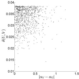
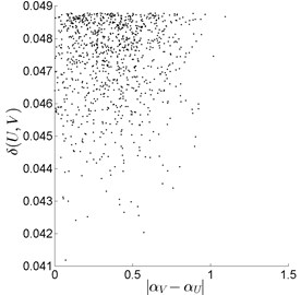
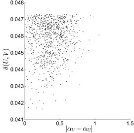
First of all, the vibration signal of rolling bearing under normal conditions (Fig. 1(a)) was processed. The 48th range fragment $U$ of size 16, the 23rd range fragment $U$ of size 32 and the 12th range fragment $U$ of size 64 were compared with all possible domain fragments $V$ of double, triple and fourfold size, respectively. Some experimental analysis results, for the case ($\left|V\right|=\text{2}\left|U\right|$), are presented in Fig. 2. As it can be seen, practically in all cases, the best pairings $\text{“}U\leftrightarrow V\text{”}$ correspond to small values of $\left|{\alpha }_V-{\alpha }_U\right|\text{.}$ For instance, the best pairing ${\text{(}\delta }_{\mathrm{m}\mathrm{i}\mathrm{n}}=\delta (U,V)=\text{0.012)}$ for the range fragment $U$ ($\left|U\right|=\text{16)}$ was fixed with $\left|{\alpha }_V-{\alpha }_U\right|\le {\epsilon }_0$, where ${\epsilon }_0=\text{0.097 (Fig. 2(a))}$. In this case, the number of potential domain fragments $V$$\text{(}\left|V\right|=\text{32)}$ decreases from 993 (brute force approach) to 215. Analogously, the best pairing $\text{“}U\leftrightarrow V\text{”}$ for the range fragment $U$$\text{(}\left|U\right|=\text{32;}$${\delta }_{\mathrm{m}\mathrm{i}\mathrm{n}}=\delta (U,V)=\text{0.041)}$was found with ${\epsilon }_0=\text{0.071}$ (Fig. 2(b)). In this case, the number of potential domain fragments $V$$\text{(}\left|V\right|=\text{64)}$ decreases from 961 to 59. Also, in Fig. 2(c), the best pairing $\text{“}U\leftrightarrow V\text{”}$ for $U$$\text{(}\left|U\right|=\text{64}$; ${\delta }_{\mathrm{m}\mathrm{i}\mathrm{n}}=\delta (U,V)=\text{0.041)}$ was fixed with $\left|{\alpha }_V-{\alpha }_U\right|\le \text{0.034,}$ and the number of potential domain fragments $V$$\left(\right|V|=\text{128})$ decreases from 897 to 11.

Fig. 2Search for best pairings “U↔V” (normal condition): a) range fragment U of size 16 (|V|= 32), b) range fragment U of size 32 (|V|= 64), c) range fragment U of size 64 (|V|= 128)

a)

b)

c)

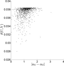
Fig. 3Search for best pairings “U↔V” (normal condition vs fault condition), with the 48th range fragment U of size 16 (|V|= 32)

a) Normal vs Ball fault

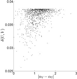
b) Normal vs Inner race fault

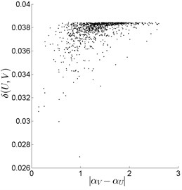
c) Normal vs Outer race fault

Secondly, the vibration signal of rolling bearing under normal condition (Fig. 1(a)) was compared with vibration signals under fault conditions (Fig. 1(b)-(d)). The same, as before, range fragments $U$ of size 16, 32 and 64 were compared with all possible domain fragments $V$ of double, triple and fourfold size, respectively. Some typical comparison results $\text{(}\left|U\right|=\text{16,}$$\left|V\right|=\text{32}$) are presented in Fig. 3.

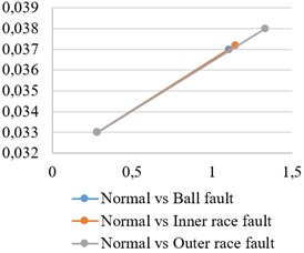
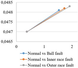
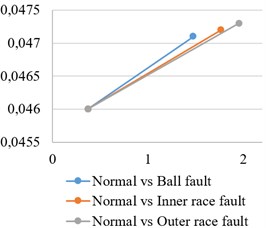
To expose differences between the two groups of searching results, “normal vs normal” (Fig. 2) and “normal vs fault” (Fig. 3), the averaged grouping (“pool”) centres $(\mathrm{\Delta }{\stackrel{-}{\alpha }}_U,\stackrel{-}{\delta })$$\text{(}∆{\alpha }_U=\left|{\alpha }_V-{\alpha }_U\right|$, $\delta =\delta (U,V$)) were found, namely $\text{(}\left|U\right|=\text{16,}\left|V\right|=\text{32):}$ (0.281, 0.033), under normal condition (Fig. 1(a)); (1.103, 0.037), under ball fault condition (Fig. 3(a)); (1.146, 0.037), under inner race fault condition (Fig. 3(b)); (1.332, 0.038), under outer race fault condition (Fig. 3(c)). As it can be seen, in the “normal vs fault” case, the “pool” centres are strongly biased to the right, in comparison with “normal vs normal” case, (Fig. 4(a)). Similar situation is observed for $\left|U\right|=\text{32}$ ($\left|V\right|=\text{64}$) and $\left|U\right|=\text{64}$ ($\left|V\right|=\text{128}$) (Fig. 4(b), Fig. 4(c)).

Based on the above considerations, we here conclude that the observable considerable displacements of “pool” centres (Fig. 4) may serve the purpose of being excellent quality criteria in the condition monitoring (gear fault diagnosis) area.

Fig. 4Location and displacement of “pool” centres: a) |U|= 16, |V|= 32, b) |U|= 32, |V|= 64, c) |U|= 64, |V|= 128

a)

b)

c)

Finally, we note that numerous experimental analysis results, associated with the same vibration signals (Fig. 1) and obtained by exploring domain fragments of triple and fourfold size (in comparison to that of range fragments), have not established any conspicuous new facts. The larger difference between the size of range and domain fragments, somewhat worse (in the mean squared error sense) pairings $\text{“}U\leftrightarrow V\text{”}$ have been detected in the signal. On the other hand, the displacement of “pool” centres was visible fairly well.

7. Conclusion and discussion

This paper presents the mathematical interpretation of the fragmentary smoothness of the vibro-acoustic signal. The smoothness of the signal is assumed to be a real number characterizing the downtrend of the spectral DT coefficients, as their serial numbers increase.

A novel iterative procedure for finding the signal smoothness parameter values (smoothness estimates) with a required degree of accuracy is proposed. The exceptionally important invariance property of the signal smoothness estimates is formulated and proved, i.e. it is shown that the signal smoothness estimate is left unchanged, as the vibro-acoustic signal is inversed or multiplied by a scalar.

In the paper, a great attention is paid to the necessary signal similarity condition. It is proved that small fragmentary changes in the vibro-acoustic signal lead to small changes in the signal smoothness parameter value. Preliminary experimental analysis results showed that the use of the necessary signal similarity condition might be of service in speeding-up some computational processes associated with fractal interpolation of vibro-acoustic signals, forecasting of real time series, detection of self-similarities in vibro-acoustic signals, early gear fault diagnosis, data mining, etc.

In particular, application of the introduced signal analysis schemes to the processing of a large number of vibration signals, associated with the gradually deteriorating condition of the rolling bearing, would necessarily facilitate computing of tolerance, risk and fault intervals for the averaged centres, discussed in Section 6. The latter centres, without any doubt, can be explored efficiently in the early fault diagnosis of the machinery.