On-line diagnosis of mechanical defects of the combustion engine with principal components analysis

1. Introduction

There is a group of mechanical defects, which – not only – are not detected by the On-Board Diagnostics (OBD) but also even camouflaged by the engine control system. As an example the pressure decrease in a cylinder, caused by a leakage of valves, rings or a head gasket puncture, can be used. Such defects cause an automatic change of control parameters, but the on-board diagnostic system does not react.

In systems of on-line diagnostics, the simple methods – which would allow to differentiate good and faulty states as well as the defects identification – are constantly searched for. When the vibration signal is recorded many diagnostic parameters can be created on its bases. A part of them is useful and provides information of the object state, a part is correlated with other data, however there is also a part which disturbs the diagnostic process. In order to select parameters carrying information the method of the Principal Component Analysis (PCA) was applied forming the empirical model allowing for an automatic classification of mechanical defects on the bases of the vibration signal. The method was described in [1] and found an application in machine diagnostics [2-5]. Several aspects of its application in diagnostics of internal combustion engines are discussed in [6-8]. Mechanical defects of the combustion engine were diagnosed by authors with other techniques: autoregressive model [9], Kalman filter [10], Singular Value Decomposition of observation subspace [11]. Condition monitoring of IC engines through the analysis of their vibrations treated as cyclostationary process is introduced in [12, 13]. Methods of vibrodiagnostics for combustion engines are discussed in [14-16]. The results of research, which aim is to diagnose damages of mechanical elements of car combustion engine using vibration signals and artificial neural networks are presented in [17]. The method described in the paper aim is to supplement – already operating in vehicles – the OBD system (which detects emission faults) with mechanical defects diagnostics [18].

2. Principal component analysis

The main purpose of principal component analysis is the reduction of the dimension of the dataset with minimal loss of information. In other words, PCA projects the original set of data into different subspace. The new coordinates are called principal components, which are uncorrelated and explain the variation in the data. The first principal component is the axis with maximum data variance as possible, and each succeeding one accounts for as much of the variability in the data as possible.

PCA can be done using eigenvalue decomposition of a data covariance matrix $\mathbf{X}$:

Each row of $\mathbf{X}$ corresponds to all $p$-measurements of a particular type and each column of $\mathbf{X}$ corresponds to a set of measurements from one test.

Eigenvalues ${\lambda }_i$ and associated with them eigenvectors ${\mathbf{w}}_i$ of ${\mathbf{R}}_{xx}$ covariance matrix are linked by:

Moreover, the eigenvectors with the largest eigenvalues form the matrix $\mathbf{W}$, which transforms data onto the new subspace:

where: $\mathbf{x}=[x_1,x_2,{\dots ,x_N]}^T$ – vector of original data, $\mathbf{y}={\left[y_1,y_2,{\dots ,y}_k\right]}^T$ – reduced vector of data, $\mathbf{W}={[w_1,w_2,\dots w_k]}^T$ – transformation matrix.

The variance for the $i$th principal component is equal to the $i$th eigenvalue of ${\mathbf{R}}_{xx}$ covariance matrix:

3. Description of experiment

Examinations were performed during road tests on the four-cylinder engine of spark ignition of Fiat Punto of 400 000 km mileage. Its technical data are listed in Table 1.

Measurement, recording and processing of vibration was done using vibration analyzer Pulse 3560 E, with accelerometers type 4393 produced by Brüel and Kjær. The accelerometer was fastened by means of a joint screwed into the engine side at cylinder 1. Accelerations of engine block vibrations were recorded for various rotational speeds and loads, in the vertical and horizontal directions, with a frequency of 65536 Hz, which means the frequency encompassing the sensor resonance frequency range. Simultaneously the crankshaft position signal, throttle position and signals from the ignition coil at 1 and 4 cylinder were recorded. Additional signals enabled the synchronisation and engine load.

Signals of about 1-minute duration were recorded during road test with a quasi-constant speed without rapid acceleration and deceleration. Investigations were performed for various defects of the engine [19]:

1) Engine with no defects,

2) Defected head gasket,

3) Increased clearance of the exhaust valve (+0.06 mm),

4) Decreased clearance of the exhaust valve (–0.06 mm),

5) Exhaust valve out of order I (small defect), optimal clearance,

6) Exhaust valve out of order I (large defect), optimal clearance.

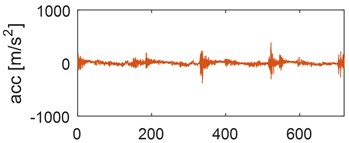
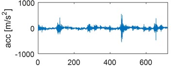
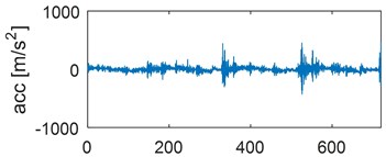
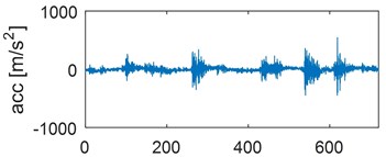
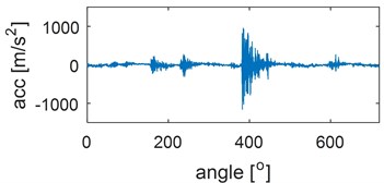
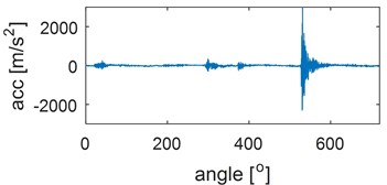
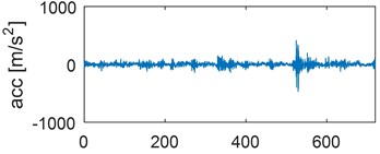
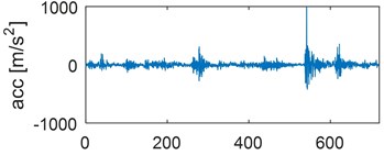
Examples of time waveforms of the acceleration of vibrations for each of the mentioned engine states for one work cycle at the rotational speed of the engine of 3000 rpm are presented in Fig. 1 and 2 (Fig. 1 – in a vertical direction, Fig. 2 – in a horizontal direction).

Fig. 1Time waveforms of vibration accelerations for engine with a) no defects, b) defected head gasket, c) defected exhaust valve (small), d) decreased clearance of exhaust valve, e) defected exhaust valve (large), f) increased clearance of exhaust valve, in vertical direction, for one work cycle at the rotational speed of the engine of 3000 rpm

a)

b)

c)

d)

e)

f)

The process of generating vibrations and noises in the internal combustion engine is very complicated. The observed vibrations are compositions of periodic waves related to operations of rotating elements and impulse responses corresponding to a piston plane-rotary motion as well as responses to gas pressure. Some excitations occur periodically, e.g. piston slap, opening and closing of valves (for engines with constant valve timing), while other are characterized by the angle variability (injection, ignition). Therefore, during the vibration measurements, the recording of additional informative and synchronizing signals, such as e.g. the engine crankshaft position is also necessary. Transient processes, being responses for valves closing, are dominating in the vibration signal recorded during the work cycle.

In order to be able to draw conclusions on the engine on-line state – under various maintenance conditions – on the grounds of vibrations, the influence of engine work parameters on the vibration signal should be investigated. The performed investigations indicate that the most important is the crankshaft rotational speed. This speed increase is accompanied by the increase of the vibration signal amplitude, especially components being the responses for valves closing.

It should be expected that the valves tightness loss would cause the effect of „whistling”. Intensification of this effect can be achieved by applying the resonance frequency range of the piezoelectric vibration sensor, which equals 55 kHz. The analogue-to-digital converter card allows the signal recording with a frequency of 65536 Hz, which enables entering into the resonance vibrations zone and to intensify the vibration response of a leaking cylinder.

Leakage in the piston-cylinder system occurs also due to burning out of the exhaust valve. The system vibration response for opening and closing of the exhaust valve is very similar to the response of the system with the increased valve clearance. Due to a resonance occurrence differentiating the valve wear degree or defects is not possible. Since the sequence of events is very important at analyzing the engine vibration signal, the time waveform should be subjected to the time windowing (time selection process). Limits of the time window must be precisely determined for each cylinder and each event (opening and closing of valves and injectors, ignition, etc.).

Increased amplitudes of vibration accelerations, when the engine runs with the defected gasket, are clearly seen in the time waveform. It can be stated, that the defect strengthens the vibration response.

Fig. 2Time waveforms of vibration accelerations for engine with a) no defects, b) defected head gasket, c) defected exhaust valve (small), d) decreased clearance of exhaust valve, e) defected exhaust valve (large), f) increased clearance of exhaust valve, in horizontal direction, for one work cycle at the rotational speed of the engine of 3000 rpm

a)

b)

c)

d)

e)

f)

4. Selection of diagnostic parameters

The described above time signals $x$ recorded during the road test became the basis for developing the observation matrix. The following parameters were applied: average value, root-mean square value (RMS), variance, the third moment of the standard score – skewness, the forth moment of the standard score – kurtosis, maximum absolute value (peak value), peak coefficient, impulse coefficient, shape coefficient. These parameters can be calculated on-line. Every parameter is determined in vertical and horizontal direction.

Since the investigated parameters are characterised by a high variability from a cycle to a cycle, the numerical filter described by the recurrent equation was applied:

Eq. (1) represents the Exponentially Weighted Moving Average Filter which is identical to a discrete first-order low-pass filter. When used as a filter, the value of ${\stackrel{-}{x}}_k$ is computed using the previous filtered value, ${\stackrel{-}{x}}_{k-1}$. The value of the filter constant, $F$, dictates the degree of filtering. Since the number of previous samples of any data sequence $p\ge$ 0, this means that 0 $\le F<$ 1. When a large number of points are being considered, $F\to \text{1}$, and ${\stackrel{-}{x}}_k\to {\stackrel{-}{x}}_{k-1}$. The Exponentially Weighted Moving Average filter places less importance to current data, which is generally noisy, and emphasizes more on the cumulative effect of older data. However, the weighting for each older data point decreases exponentially [20].

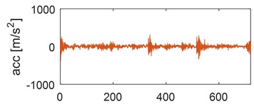
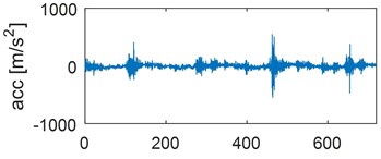
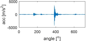
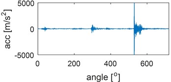
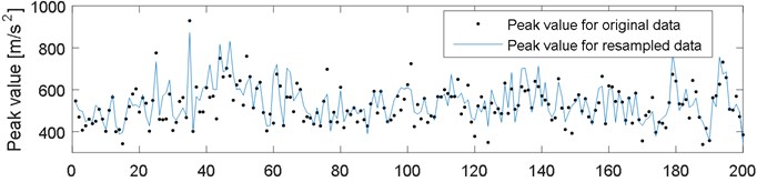
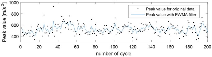
Variations of a maximum absolute value (peak value) calculated for successive 200 cycles of engine works are presented in Fig. 3. This parameter was compared with the original data and resampled into the crankshaft angle domain (Fig. 3(a)). Points in Fig. 3(b) denote peak value calculated for the original data, while a continuous line denotes values after recalculation by the EWMA filter with a factor $F=$0.6.

Fig. 3Comparison of peak value for a) original and resampled data, b) original data and data filtered with EWMA filter, during 200 working cycles of combustion engine

a)

b)

Since it is easier and faster to calculate on-line diagnostic parameters for the original data in the time domain, without their previous resampling, and the analysis indicated negligible errors at small fluctuations of rotational speeds, further operations were performed on the vibration signals in the time domain.

Averaged parameters values for 200 cycles are listed in Table 2, with a confidence range being within the threefold value of the standard deviation. Central moments of higher orders (from 3 to 6) were also calculated but since the scatter of these parameters was several times exceeding their values the authors resigned from them, at the stage of the primary selection already. Parameters in Table 2 are written in a sequence of increasing relative scatter value for the given parameter, taking into account mainly the good engine condition.

The matrix of training parameters $\mathbf{X}$, which columns constituted vectors of diagnostic parameters calculated in horizontal and vertical direction for one cycle of engine work, and rows – parameters in successive 200 measuring cycles for each engine state (1 no-fault state and 5 damage states mentioned above). In such way the matrix 18×1200 was obtained. Then the covariance matrix of training parameters was estimated from the mean centered data matrix:

On account of the domination of the first two eigenvalues ${\lambda }_1$ and ${\lambda }_2$ over the remaining ones, in further analysis the first two rows of the matrix $\mathbf{W}$ were used. It means the first two main components $y_1$ and $y_2$, determined from Eq. (3).

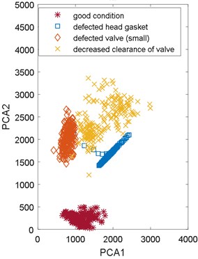
The classification of engine defects based on two main components which explain 87 % of the variation is presented in Fig. 4.

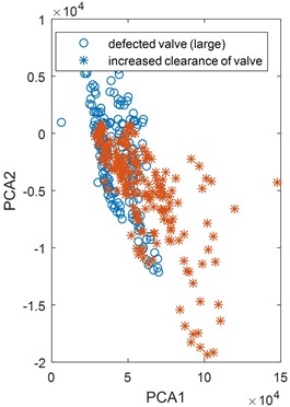
Four classes corresponding with technical states of the vehicle: no-fault state, decreased valve clearance, engine head gasket damaged, exhaust valve initial damage – are presented in Fig. 4(a). When the exhaust valve damage is growing the main components are changing, getting near and even overlapping factors obtained for the increased valve clearance (Fig. 4(b)).

The classification was performed by the Support Vector Machine (SVM) method and 99.1 % of hits was achieved. In machine learning, support vector machines are supervised learning models with associated learning algorithms that analyze data and recognize patterns, used or classification and regression analysis. Given a set of training examples, each marked for belonging to one of two categories, an SVM training algorithm builds a model that assigns new examples into one category or the other, making it a non-probabilistic binary linear classifier. An SVM model is a representation of the examples as points in space, mapped so that the examples of the separate categories are divided by a clear gap that is as wide as possible. New examples are then mapped into that same space and predicted to belong to a category based on which side of the gap they fall on. The method is described in [3, 21, 22].

Fig. 4Classification of engine defects based on PCA, a) good technical condition, defected head gasket, defected exhaust valve (small), decreased clearance of exhaust valve, b) increased clearance of exhaust valve and defected exhaust valve (large)

a)

b)

It results from the analysis that the highest fraction in main components have variance and peak value. The procedure of selecting coefficients of the model Eqs. (1)-(3) was repeated for four parameters of the highest influence on the main components. For the new reduced model, the classification results improved and equals now 99.3 % of correct hits for damages.

Thus – in the proposed method – vectors ${\mathbf{w}}_1$ and ${\mathbf{w}}_2$ constitute the empirical diagnostic model of the engine. Their values are shown in [23].

The classification results were verified for the next 200 work cycles of the engine for 4 states: 1 – no-fault state, 2 – engine head gasket damage, 3 – exhaust valve initial damage, 4 – decreased valve clearance (Table 3). The engine no-fault state is recognised in 100 %. When there is a gasket damage 1 sample is recognised as a defective valve and 3 samples as a decreased valve clearance.

Finding of the model which would allow to differentiate all states was not achieved at this stage of the classification. Thus, two states which cannot be differentiated should be treated as one class of damage.

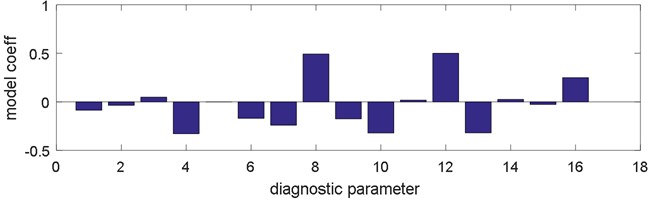
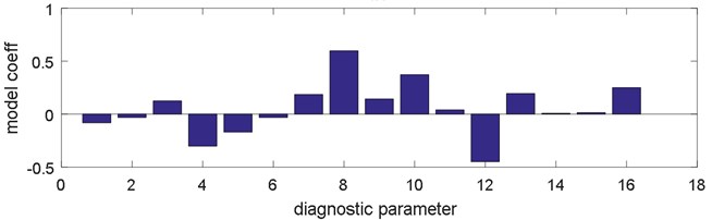
At the second stage of the classification it was attempted to differentiate the state of increased valve clearance and the state of exhaust valve damage. Since the signal variance for these states is characterised by a large relative scatter value the procedure of the model coefficients determination according to Eqs. (1)-(3) was performed for 16 remaining parameters. The obtained classification result was 100 %. The classification of two engine defects (large defect of the exhaust valve and enlarged clearance of exhaust valve) based on two main components is presented in Fig. 5. Values of empirical diagnostic model for second stage classification shown in Fig. 6. In this case all parameters are taken into account during calculations of principal components.

Fig. 5Classification of engine defects based on PCA for increased clearance of exhaust valve and large defect of exhaust valve

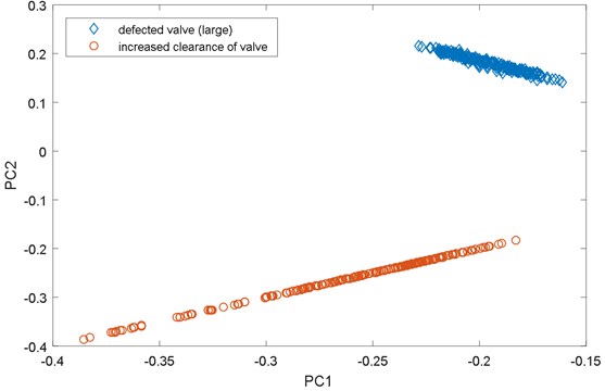
Fig. 6Model coefficients a) for 1. principal component, b) for 2. principal component; (Parameters: 1, 2 – average value (vertical, horizontal), 3, 4 – skewness, 5, 6 – kurtosis, 7, 8 – variance, 9, 10 – peak value, 11, 12 – peak coefficient, 13, 14 – impulse coefficient, 15, 16 – shape coefficient

a)

b)

5. Conclusions

The method of the preliminary recognition of defects of the internal combustion engine, which was verified for the Fiat Punto engine with spark ignition, is presented in the hereby paper. The method uses statistic parameters of the engine vibration signal. Since it was noticed – when this method is applied – that resampling does not influence the classification result the original time signal can be used. This influences the implementation easiness and calculation speed, which is important during on-line diagnostics.

During the preliminary selection of diagnostic parameters, the parameters – which scatter exceeded the parameter values for the engine in a serviceable state – were eliminated. The PCA method was applied in order to reduce the diagnostic parameters vector. The influence of individual parameters on fractions of main components was analysed. The information redundancy was eliminated. It was pointed out that for the reduced vector of diagnostic parameters the classification result is even better than for the full vector taken into consideration previously. It was considered preliminarily to broaden the vector of parameters with central moments of higher degrees but this idea was abandoned due to a large variability of engine work cycles, which would cause an increased scatter of parameters inside the class and worsening of the classification quality. Scatters within classes can be decreased by increasing the value of factor $F$ of EWMA filter, loosing simultaneously instantaneous parameters changes. Finally, the empirical statistic model was developed, taking into account 2 diagnostic parameters – variance and peak value in vertical and horizontal direction multiplied by weigh coefficients selected by means of the PCA method. This model allows to differentiate the no-fault engine technical state from 4 damage states with more than 99 % certainty. Since the attempt of finding such principal components which would allow to differentiate all 6 states was not successful, two states remained in the first stage should be treated as one defect. In the next stage their differentiation occurs, also by means of the Principal Component Analysis.

The model can be further developed to be suitable for recognition of other damages. The method was elaborated with the idea of supplementing the OBD system with the mechanical damages recognition on the basis of the vibroacoustic signal.