Abstract
In this paper, a method based on wavelet support vector machine (SVM) with OAOT algorithm, multi-layer perceptron (MLP) and Morlet wavelet transform were designed to diagnose different types of fault in a gearbox. A scale selection criterion based on the maximum relative energy to Shannon entropy ratio is proposed to determine optimal decomposition scale for wavelet analysis. Moreover, energy and entropy of the wavelet coefficients are used as two new features along with other statistical parameters as input of the classifier. The results showed that the WSVM identified the fault categories of gearbox more accurately as compared to the MLP network.
1. Introduction
The condition monitoring of gearboxes with vibration signal has been an interesting topic for researchers in this field. Therefore, recently fault diagnostics and monitoring methods for gearboxes have been improved. With the improvement of condition monitoring devices, the fault diagnosis systems tended toward the real-time fault detection methods. The real-time processing systems are mostly unable to process several vibration signal input features. Therefore, it was desired for the fault diagnosis systems to collaborate with feature selection algorithms to increase the efficiency of fault detection and decrease the human errors. The following section is comprised of an introduction to gearbox fault detection systems and feature selection techniques, based on artificial neural networks (ANNs), fuzzy systems and the genetic algorithm. Continuous wavelet transform (CWT), as a time-frequency representation of signal, provides an effective tool for vibration-based signal in fault detection. CWT provides a multi-resolution capability in analyzing the transitory features of non-stationary signals. Behind the advantages of CWT, there are some drawbacks; one of these is that CWT provides redundant data, so it makes feature extraction more complicated. Due to this data redundancy, data mining and feature reduction are extensively used, such as decision neural network as a classifier has been applied to machine health diagnosis, for example, for classifying rotating machines with imbalance and rub faults [1], bearing faults [2]. Bartelmus and Zimroz [3] successfully performed fault detection in multi-stage gearboxes by taking into account information about variations in speed and load. On the other hand, there are approaches that exploit the non-stationary character of the vibration signals generated by mechanical drives operating under variable conditions. Baydar and Ball [4] performed detection of gear deterioration under different loads using instantaneous power spectrum by employing Wigner–Ville distribution (WVD). They successfully performed fault detection of gear faults irrespective of the variable operating conditions. Fan and Zuo [5] combined Hilbert and wavelet packet transforms for detection of gear faults. Samantha and Balushi [6] have presented a procedure for fault diagnosis of bearings by ANNs. Paya et al. [7] used from wavelet transform and back propagation artificial neural network for fault diagnosis of gears and bearings. Tse et al. [8] for selection of the best wavelet family member and reduction of data redundancy presented the exact wavelet analysis for fault diagnosis of a gearbox. In Tabriz University, fault diagnosis of a gearbox was done by MLP neural network [9]. Rafiee et al. [10] selected four statistical features and studied 324 mother wavelets and then showed that the db44 wavelet is the most effective for fault diagnosis of a four-speed motorcycle gearbox. Kankar et al. [11] considered seven different base wavelets for fault detection in roller bearings and complex Morlet wavelet was selected based on the minimum Shannon entropy criterion. They also considered six base wavelets in which three are from real values and three from complex values [12]. Rafiee et al. [13] optimized the parameters of the WPT with Daubechies wavelet function and number of neurons in the hidden layer of a MLP for fault diagnosis of a gearbox. They used from standard deviation of the wavelet packet coefficients for input layer of MLP. Kankar et al. [14] conducted a comparative study of the effectiveness of artificial neural network and support vector machine in fault diagnosis of bearings. The results show that the classification with SVM is better than of ANN. The use of Daubechies wavelet and MLP back propagation artificial neural network for fault classification of a gearbox has been studied by Saravanan and Ramachandran [15]. Nikolaou and Antoniadis [16] have used wavelet packet transform to identify the nature of rolling element bearing faults. Prabhakar et al. [17] and Purushotham et al. [18] have used discrete wavelet transform for detection of bearing race faults. Chen et al. [19] used from CNN and linear SVM for gearbox fault identification and classification.
Regarding the references, neural networks can be effectively used in the diagnosis of various gear faults, but in this study, MLP and WSVM are utilized for classification. In addition, two new neurons are considered as inputs of the network to enhance the accuracy of the MLP and WSVM.
This paper is arranged as the following eight sections. Section 1 is the introduction of research background; Section 2 is about CWT review; Section 3 expounds the methodology and technology of feature extraction, in addition in this section we describe the optimal scale; Section 4 is about two classifiers method. Section 5, discusses the experimental dataset of Shahrekord University gearbox. In Section 6, modeling and designing frameworks of MLP and WSVM is described; Section 7 is about the detail of fault diagnosis method and the conclusion and discussion are expressed in Section 8.
2. Morlet wavelet transform (MWT)
If there exists a function whose Fourier transform () satisfies the admissibility condition:
We define the function mother wavelet. The corresponding wavelet family consists of a series of son wavelets, which is generated by dilation and translation operations from the mother wavelet shown as follows:
In Eq. (2), parameters and are the scale factor and , time location respectively, the term is used to ensure energy preservation. The continuous wavelet transform of a signal is defined as follows:
where is the conjugate of . In practice, the signal is of discrete form and the transformation result is a series of coefficients with the same length as the original signal. The CWT at scale can be considered as scanning the signal by changing its time location , and the coefficients essentially express the similarity between the signal and the mother wavelet. This feature of the wavelet transform can be indicated by any mother wavelet, such as Morlet wavelet, which is defined as:
For a real signal, the real part of the Morlet function is used as follows:
Through dilation and translation operations, we have a family of Morlet wavelets as:
Eq. (6) is defined by four parameters: , , and . Parameter adjusts the envelope of the wavelet function. Increasing the value of will decrease the frequency resolution of the wavelet function while increasing its time resolution [20].
3. Feature extraction
In fault diagnosis methods, the statistical values are calculated from vibration signal to construct feature vectors which are directly input into the diagnosis model for gearbox fault diagnosis. For fault diagnosis of the gearbox in this paper, time domain features are extracted to recognize various gearbox fault conditions. They are standard deviation (STD), kurtosis (KUR), shape factor (SF), skewness (SKW), impulse factor (IF) and root mean square (RMS). Time-domain features are extracted from MWT of each of the collected vibration signals. These features will be input into a WSVM and MLP to automatically identify the health conditions of the gearbox.
3.1. Optimum scale of MWT
For feature reduction, the optimal amounts of scales should be extracted. Wavelet entropy and energy are used to select the optimal scale of the basic Morlet wavelet. The proper scale is chosen when the Shannon entropy of the corresponding wavelet coefficients is minimum and the energy is maximum. A combination of the energy and Shannon entropy content of a signal’s wavelet coefficients is named by energy to Shannon entropy ratio [21] and is presented by:
Generally, the energy associated with wavelet coefficient at each scale is calculated as:
where is the length of wavelet coefficients and represents the wavelet coefficient at scale . The total energy of a signal is given by:
A normalized value, called relative wavelet energy, can be defined as:
In Eq. (11), represents the energy probability distribution across all the scales. Eq. (12) gives the entropy of signal wavelet coefficients:
4. Classifiers
4.1. Multi-layer perceptron
A multilayer perceptron (MLP) is a feed forward artificial neural network that maps sets of input data on to a set of outputs. An MLP consists of multiple layers of nodes in a directed graph, with each layer fully connected to the next one. Except for the input nodes, each node is a neuron with a nonlinear activation function. MLP utilizes a back propagation method for training of the net. Learning occurs in the perceptron by changing connection weights after each piece of data is processed, based on the amount of error in the output compared to the expected result. This is an example of supervised learning, and is carried out through back propagation, a generalization of the least mean squares algorithm in the linear perceptron. We represent the error in output node in the nth data point by , where is the target value and is the value produced by the perceptron. We make corrections to the weights of the nodes based on those corrections which minimize the error in the entire output, given by:
The change in each weight is as follows:
In the Eq. (13), and are the output of the previous neuron and learning rate respectively, which is carefully selected to ensure that the weights converge to a response fast enough, without producing oscillations. The derivative to be calculated depends on the induced local field , which it varies. It is easy to prove that for an output node this derivative can be simplified to:
where is the derivative of the activation function described above, which itself does not vary. The analysis is more difficult for the change in weights to a hidden node, but it can be shown that the relevant derivative is:
This depends on the change in weights of the th nodes, which represent the output layer. So, to change the hidden layer weights, we must first change the output layer weights according to the derivative of the activation function, and so this algorithm represents a back propagation of the activation function [22].
4.2. Wavelet support vector machine
The wavelet function can be defined as:
where , , , a is a dilation factor, and c is a translation factor. If is the wavelet function of 1D, the multi-dimensional wavelet function can be defined using tensor theory as:
where and, is the dimension number. Let denotes a mother kernel function. Then dot-product wavelet kernels are:
The decision function for classification is:
where the denotes the th component of the th training example. The Mexican hat mother wavelet is , and the corresponding wavelet kernel function is:
Morlet wavelet kernel is a support vector kernel function. It is defined as follows:
The corresponding wavelet kernel of Morlet function is:
In this paper, four kernel functions are used: wavelet Morlet, wavelet Maxican hat, Gaussian wavelet kernel and wavelet Shannon. In this paper, the multi-class classification strategy, such as OAOT [23] with different wavelet kernel functions is used for classification.
5. Gearbox dataset
The experimental test rig at Shahrekord University of Iran to collect dataset consists of a gearbox with spur gears, a flywheel and an electrical motor. Electrical motor, gearbox and flywheel are attached together through flexible couplings as shown in Fig. 1. Vibration signals are collected by mounting the accelerometer on the top of the gearbox. “Easy Viber” data collector and its software, “SpectraPro”, are used for data acquisition. The signals are sampled at 16 KHz lasting 4 sec. In the present study, four pinion wheels whose details are as mentioned in Table 1 are used. One wheel is new one and is assumed to be free from defects. In the other three pinion wheels, defects are created. The raw vibration signals acquired from the gearbox when it is loaded with various pinion wheels discussed above. The vibration signal from the piezoelectric transducer (accelerometer) is captured for the following conditions: good gear, gear with tooth breakage, chipped gear and eccentric gear. For bearing vibration signal acquisition four ball bearings whose details are as mentioned in Table 2 are used. One new bearing is considered as good bearing. In the other three bearings, some defects are created and then various bearings are installed and the raw vibration signals acquired on the bearing housing. So, the vibration signals are captured for the following conditions: good bearing, inner race fault, outer race fault, ball fault in bearing and bearing with combine defect.
Fig. 1Experimental test setup [21]
![Experimental test setup [21]](https://static-01.extrica.com/articles/16813/16813-img1.jpg)
Table 1Gear wheel and pinion details
Parameters | Pinion wheel | Gear wheel |
Outer diameter | 63 | 93 |
No. of teeth | 40 | 60 |
Module | 1.5 | 1.5 |
Normal pressure angle | 20° | 20° |
Top clearance | 0.3 mm | 0.3 mm |
Material | C.K 45 | C.K 45 |
Table 2Bearing details
Description | Self-aligning ball bearing |
Designations bearings with tapered bore | 1209K |
Outer diameter | 85 |
Inner diameter | 45 (taper1:12 in diameter) |
Each set of faults was tested under five variable rotational speeds of the input shaft until 30, 35, 40, 45 and 50 Hz.
6. Modeling of gearbox condition using MLP and WSVM
The fault diagnosis system which is modelled by both MLP and WSVM has 9 inputs and the output layer has 8 neurons, one for each condition of the gearbox to classify. The input variables ( to ) of the system are the feature of continues wavelet coefficient such as standard deviation (STD), skewness (SKW), kurtosis (KUR), shape factor (SF), impulse factor (IF) and root mean square (RMS), rotor speed (RS), energy (E) and Shannon entropy (SE) of the Morlet wavelet coefficients of vibration signals. The inner race fault, outer race faults, ball faults, combined faults, chipped gear, broken gear, eccentric and healthy gearbox conditions. We have used from MATLAB 6.5 standard software for training and testing of all network. The dataset for the efficiency of system available included 85 data patterns for each. From these, 70 % data patterns were used for training the MLP and WSVM, and the remaining 30 % patterns were used as the test dataset. The architecture and training parameters for MLP and WSVM are listed in Table 5. In this paper, a dataset containing not only the different fault categories and severities but also the compound faults are analyzed. Table 3 represents the eight conditions for gearbox and consists of 680 samples. The 680 data samples are divided into 440 training and 240 testing instances. We map each term of input data of the network to a value between –1 and 1 for hyperbolic tangent function and between 0.1 and 0.9 for sigmoid function using the following linear mapping formula:
where is normalized value of the real variable; –1 or 0.1 and 1 or 0.9 are minimum and maximum values of normalization, respectively; is real value of the variable; and are minimum and maximum values of the real variable, respectively. The sigmoid function is most useful for training a set of data that is saturated between 0 to 1 because the sigmoid activation function will produces a positive numbers between 0 to 1. Hyperbolic tangent activation function is categorized in the logistic family similar to the sigmoid function and the output value saturated between –1 to +1. These normalized data were used as the inputs to train the MLP and WSVM. The normalization of the input values will increase the numerical stability of the neural network processing. The value of output nodes represents the training target of neural network: “l” means failure and “0” means normal. So, the output is represented as [0 0 0 0 0 0 0 0] for normal, [1 0 0 0 0 0 0 0] for fault with label 1 (CG), [0 1 0 0 0 0 0 0] for fault with label 2 (BG) and [0 0 0 0 0 0 1 0] for fault with label 7 (BCF).
The topology of MLP and WSVM has been shown in Fig. 2.
Table 3Gearbox condition
Condition | Abbreviation | Label |
Healthy gearbox (HG) | 0 | |
Chipped gear (CG) | 1 | |
Broken gear (BG) | 2 | |
Eccentric gear (EG) | 3 | |
Bearing with ball fault (BBF) | 4 | |
Bearing with fault in outer race (BORF) | 5 | |
Bearing with fault in inner race (BIRF) | 6 | |
Bearing with combined fault (BCF) | 7 |
The most common activation function are linear, sigmoid function (Logsig) and hyperbolic tangent sigmoid function (Tansig). Table 4 shows the expression of activation function of MLP.
The choice of activation functions for each layer is commonly based on experience of researchers. In this study, sigmoid, hyperbolic tangent sigmoid and linear functions are investigated in the hidden layer of the MLP. The choice of training parameters is sometimes critical to the success of the neural network training process. Unfortunately, the choice of these values is generally problem dependent. There is no generic formula that can be used to choose these parameter values. The network training is also limited to 10000 epochs and the validation dataset may affect the training, with a maximum of 1000 iteration failed. In this work, network training is finished when either the root mean-square error of the training dataset or the change in network error is less than 0.005. The initial weights of the neural network play a significant role in the convergence of the training method. Without a priori information about the final network weights, it is common practice to initialize all weights with random numbers of small absolute values between [–0.01, 0.01]. The learning rate used in this case was 0.9 for MLP. For ANN, the back propagation learning algorithm with single hidden layer has been used. The other parameters of MLP is given in Table 5.
Fig. 2The MLP structure
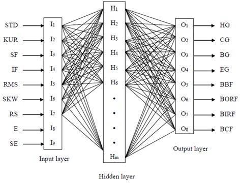
Table 4Activation function used in MLP neural network
Activation function | Output equations |
Linear | |
Sigmoid | |
Hyperbolic tangent |
Table 5Parameters of MLP
Network | MLP |
Number of hidden layers | 1 |
Activation functions | Tansig, Logsig, Linear |
Training method | Back propagation |
Mean squared error goal | 1e-5 |
Max epochs | 10000 |
Learning rate | 0.85 |
The initial weight and biases | Random |
Number of neuron in hidden layers | Varied from 5 to 30 |
Number of neurons in input layer | 9 |
Number of neurons in output layer | 8 |
Momentum learning step size | 0.9 |
Momentum learning rate | 0.9 |
Network input distribution (training) | 70 % |
Network input distribution (testing) | 30 % |
We construct wavelet SVM using four wavelet functions and then input training set into network and train the network. Mean squared error (MSE) is a SVM performance function. It measures the SVM performance according to the mean of squared errors. The MSEs of each function are shown in Table 6. From Table 6, we can draw the conclusion that running time and MSE of Morlet function in the hidden layer is the best in compare to other functions. The results, in this paper, are consistent with the fact that most papers adopt Morlet as mother wavelet functions to construct wavelet neural network [22]. So, we can use Morlet wavelet functions to create WSVM.
Table 6Predicting results of different mother wavelet function for WSVM
Wavelet function | Morlet | Mexican hat | Gaussian | Shannon |
MSE | 1.012e-3 | 4.37e-2 | 1.98e-3 | 14.23e-2 |
Running time (s) | 46.74 | 58.90 | 69.65 | 50.52 |
Table 7 shows the performance of MLP with different activation function. From Table 7, it is clear that tansig activation function is the best performance in compare to other activation functions that we have used in the MLP NN.
Table 7Predicting results of different activation function for MLP
Activation function | Linear | Logsig | Tangsig |
MSE | 11.01e-3 | 5.14e-3 | 3.34e-3 |
Running time (s) | 38.90 | 33.67 | 22.56 |
7. Results and discussions
In this paper the six different base wavelets are considered in which three are from real valued (Meyer, Coiflet5 and Symlet2) and other three from complex valued (complex Gaussian, complex Morlet and Shannon wavelets). Out of these six wavelets, the base wavelet is selected based on wavelet selection criterion to extract statistical features from wavelet coefficients of raw vibration signals. The wavelet selection criteria Maximum Relative Wavelet Energy is used to select an appropriate wavelet for feature extraction. The Complex Morlet wavelet is selected based on Maximum Relative Wavelet Energy criterion. In the present study, training and testing of the classifiers as MLP and WSVM have been carried out. The CWC of vibration signals are calculated using complex Morlet wavelet. The complex-valued Morlet wavelet “cmor1-0.5” is selected as the base wavelet. The bandwidth of the wavelet is set as 1, and the center frequency of the wavelet is chosen as 0.5. The scales investigated were 1-128. In this paper, as shown in Section 3.1, for feature reduction, the optimal scale is extracted based on wavelet entropy and energy. The optimal scale is chosen when the Shannon entropy of the corresponding wavelet coefficients is minimum and the energy is maximum. So, the distribution of energy to Shannon entropy belongs to each scale level from scale 1 to 128 for healthy condition of pinion is shown in Fig. 3. The optimal scale with this criterion is 42.29. In addition, we have done this procedure for bearing condition of the Shahrekord test rig and we have found the optimum scale for bearing conditions is 4.9.
In this paper, the statistical parameters, energy and Shannon entropy in optimal scale are used for input data of MLP and WSVM. The number of hidden layers and hidden nodes affect both the network accuracy and the time required to train the neural network. The hidden layers, basically, provide the networks ability to generalize performance of outputs. In most cases, one or sometimes two hidden layers are used. In this study one hidden layer is chosen for MLP. The adequate number of hidden units depends on many factors. Some of them are number of training patterns, number of input and output units, type of activation function, training algorithm. When too few hidden units used, generally results in high training error due to under fitting. When too many used, obviously results in low training errors, but will make training unnecessarily slow. There is not a general procedure for selecting the optimum number for hidden units. The reasonable strategy is to try a series of hidden units and find a number which works best. In this study, the maximum number of hidden unit is chosen to be thirty and decreased to investigate effect on accuracy. In order to perform an objective comparison of various neural networks, it is of interest to set the number of hidden nodes between 5 to 30 for different tests. So, it was found by trial and error that 24 neurons in the hidden layer of MLP, can give model, which have the best performance in the verification stage. Table 8 shows the effect of the number of hidden neurons on the MLP performance. It is clear that although adding more than 24 hidden neurons make the mean square error (MSE) training smaller, this deteriorates network’s generalization capabilities with increasing the average verification errors instead of decreasing them. Therefore, the optimum number of the MLP is 24 neurons.
Fig. 3The relation between energy to Shannon entropy ratio and scale for pinion with MWT
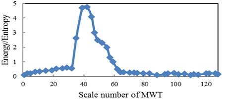
Table 8The effects of different number of hidden neurons on the MLP performance
Number of hidden neurons | Average error (%) in fault diagnosis with MLP | RMS error (MLP) | Training epochs |
5 | 25.37 | 0.014314 | 9887 |
8 | 24.39 | 0.022527 | 8647 |
10 | 23.30 | 0.027632 | 5489 |
12 | 22.29 | 0.050432 | 5034 |
15 | 19.45 | 0.091621 | 4065 |
18 | 18.22 | 0.072543 | 3009 |
20 | 18.10 | 0.013274 | 3721 |
22 | 17.19 | 0.032932 | 2941 |
24 | 16.67 | 0.085132 | 5078 |
30 | 24.47 | 0.016521 | 8340 |
Tables 9 and 10 show the performance of the WSVM with Morlet kernel and MLP classifier for gearbox fault diagnosis is acceptable. The results of Table 10 are accordance with 24 neurons in the hidden layer. From Tables 9 and 10, we found that the WSVM has better accuracy in classification of gearbox faults in comparison of MLP. In Tables 9 and 10, Tr. A., Te. A., and T. T., are training accuracy, testing accuracy and training time respectively.
Table 9WSVM classification performance for Shahrekord test rig
Performance | Gear faults | Bearing faults | ||||||
Healthy | Chipped | Broken | Eccentric | Inner | Ball | Outer | Combine | |
Tr. A. (%) | 100 | 93.33 | 100 | 93.33 | 100 | 100 | 100 | 93.33 |
Te. A. (%) | 100 | 86.66 | 93.33 | 86.66 | 86.66 | 93.33 | 93.33 | 86.66 |
Overall accuracy (%) | 90.82 | |||||||
T. T.(s) | 46.74 | |||||||
We compared the performance of the presented wavelet kernel SVM with Gaussian, Morlet, Mexican hat and Shannon. Classification results using these kernel are shown in Table 11. From Table 11, it is clear, the SVM with Morlet wavelet function has the highest accuracy point (90.82 %) among the other wavelet functions. In Table 11, parameter C is error/margin trade off.
Table 10MLP classification performance for Shahrekord test rig
Performance | Gear faults | Bearing faults | ||||||
Healthy | Chipped | Broken | Eccentric | Inner | Ball | Outer | Combine | |
Tr. A. (%) | 100 | 86.66 | 93.33 | 86.66 | 93.33 | 86.66 | 93.33 | 86.66 |
Te. A. (%) | 93.33 | 80.00 | 86.66 | 73.33 | 86.66 | 80.00 | 86.66 | 80.00 |
Overall accuracy (%) | 83.33 | |||||||
T. T. (s) | 22.56 | |||||||
Table 11Comparison among four wavelet kernels for fault classification with OAOT
Method | Kernel | Kernel parameter | C | Accuracy (%) |
OAOT | Gaussian | 4 | 10 | 86.54 |
OAOT | Mexican hat | 0.95 | 15 | 87.78 |
OAOT | Shannon | 3 | 102 | 88.34 |
OAOT | Morlet | 0.88 | 55 | 90.82 |
Table 12A comparison between the present work and some recent publications
Reference | Objects | Defects | Vibration signal | Techniques for vibration signature analysis | Features | Classifier |
Paya et al. [7] | ||||||
Nikolaou and Antoniadis [16] | Bearings and gears | Inner race of bearing and gear tooth irregularity | Stationary | Daubechies 4 | Time and frequency and their amplitudes | ANN |
Prabhakar et al. [17] | Rolling element bearings | Inner race, outer race | Stationary | Daubechies 4 | RMS, KUR | NA |
Purushotham et al. [18] | Rolling element bearings | Inner race, outer race, ball fault and combination of faults | Stationary | Daubechies | Mel frequency complex cepstrum (MFCC) coefficients | Hidden Markov model |
Saravanan et al. [15] | Gears | Gear tooth breakage, gear with crack at root and with face wear | Stationary | Morlet wavelet | STD, VAR, KUR and minimum value | SVM and proximal SVM |
Rafiee et al. [9] | Gears and bearings | Slight-worn, medium- worn and broken tooth for gear, only faulty bearings | Stationary | Daubechies 4 | STD | ANN |
Rafiee et al. [10] | Gears and bearings | Ball, cage, inner race, outer race defects on bearings and slight-worn, medium- worn and broken tooth for gear | Stationary | 324 mother wavelets | VAR, STD, KUR and 4th central moment of CWC- SV | ANN |
Chen et al. [19] | Gears and bearings | Gear with face wear, pitting and breakage, and inner, outer and ball fault of bearing | Stationary | FFT | STD, KUR, SKW and mean | CNN, SVM |
Present work | Gears and bearings of gearbox | Refer to table 3 (8 conditions for gearbox) | Non-stationary | Six base wavelet with two wavelet section criteria (Complex Morlet) | STD, KUR, SF, RMS, SKW, RS, E, SE (refer to figure 2) | MLP and wavelet SVM |
From the above discussion, we find that the use of Morlet wavelet and extraction of statistical features from the wavelet coefficients were found to be very efficient for classification using MLP and WSVM. Optimal scale method is a good tool in selecting the best features among the extracted feature vectors. The accuracy of calcification with MLP and WSVM are 83.33 % and 90.82 %, respectively. From Tables 9 and 10, we can see that WSVM and MLP are very close in classification capability, but the time required for training and classification using WSVM is more compared to MLP technique and taking this into account the authors claim that WSVM has upper hand over MLP. To show the efficiency of the selected features and the methodology, a comparison between the current work and some published literatures has been shown in Table 12. In this table, comparison has been made on the basis of the objects used, defects considered for the study, techniques used for vibration signature analysis, features considered, classifier used and the classifier efficiencies in each paper.
8. Conclusions
In this paper, a method for fault diagnosis of gearbox faults has been presented based on combining continuous wavelet, MLP and WSVM. Morlet wavelet was used and the statistical features from the wavelet coefficients were extracted. To find very efficient features for classification, maximum energy to Shannon entropy ratio was employed to search for the optimal scale of CWT and consequently the features were reduced. This feature reduction method improved the performance of the classifiers in fault detection. As a new idea, energy and Shannon entropy have been applied as two new features along with statistical parameters as input of the classifier. The obtained results indicate that the accuracy of the classifier has been increased between 5 to15 percentage points by considering these two features.
References
-
Mc Cormick A. C., Nandi A. K. Classification of the rotating machine condition using artificial neural networks. Proceedings of the Institution of Mechanical Engineers, Vol. 211, 1997, p. 439-450.
-
Li B., Chow M., Tipsuwan Y., Hung J. C. Neural network based motor rolling bearing fault diagnosis. IEEE Transactions on Industrial Electronics, Vol. 47, Issue 5, 2000, p. 1060-1069.
-
Bartelmus W., Zimroz R. A new feature for monitoring the condition of gearboxes in non-stationary operating conditions. Mechanical Systems and Signal Processing, Vol. 23, Issue 5, 2009, p. 1528-1534.
-
Baydar N., Ball A. Detection of gear deterioration under varying load conditions using the instantaneous power spectrum. Mechanical Systems and Signal Processing, Vol. 14, Issue 6, 2000, p. 907-921.
-
Fan X., Zuo M. J. Gearbox fault detection using Hilbert and wavelet packet transform. Mechanical Systems and Signal Processing, Vol. 20, Issue 4, 2006, p. 966-982.
-
Samantha B., Al-Balushi K. R. Artificial Neural Networks based fault diagnostics of rolling element bearings using time domain features. Mechanical Systems and Signal Processing, Vol. 17, Issue 2, 2003, p. 317-328.
-
Paya B. A., Esat I. I., Badi M. N. M. Artificial neural network based fault diagnostics of rotating machinery using wavelet transforms as a preprocessor. Mechanical Systems and Signal Processing, Vol. 11, Issue 5, 1997, p. 751-765.
-
Tse P. W., Yang W. X., Tam H. Y. Machine fault diagnosis through an effective exact wavelet analysis. Journal of Sound and Vibration, Vol. 277, Issues 4-5, 2004, p. 1005-1024.
-
Rafiee J., Arvani F., Harifi A., Sadeghi M. H. Intelligent condition monitoring of a gearbox using artificial neural network. Mechanical Systems and Signal Processing, Vol. 21, Issue 4, 2007, p. 1746-1754.
-
Rafiee J., Rafiee M. A., Tse P. W. Application of mother wavelet functions for automatic gear and bearing fault diagnosis. Expert Systems with Applications, Vol. 37, Issue 6, 2010, p. 4568-4579.
-
Kankar P. K., Sharma S. C., Harsha S. P. Fault diagnosis of ball bearing using continuous wavelet transform. Applied Soft Computing, Vol. 11, Issue 2, 2011, p. 2300-2312.
-
Kankar P. K., Sharma S. C., Harsha S. P. Rolling element bearing fault diagnosis using wavelet transform. Neurocomputing, Vol. 74, Issue 10, 2011, p. 1638-1645.
-
Rafiee J., Tse P. W., Harifi A., Sadeghi M. H. A novel technique for selecting mother wavelet function using an intelligent fault diagnosis system. Expert Systems with Applications, Vol. 36, Issue 3, 2009, p. 4862-4875.
-
Kankar P. K., Sharma S. C., Harsha S. P. Fault diagnosis of ball bearings using machine learning methods. Expert Systems with Applications, Vol. 38, Issue 3, 2011, p. 1876-1886.
-
Saravanan N., Ramachandran K. I. Incipient gearbox fault diagnosis using discrete wavelet transform (DWT) for feature extraction and classification using artificial neural network (ANN). Expert Systems with Applications, Vol. 37, Issue 6, 2010, p. 4168-4181.
-
Nikolaou N. G., Antoniadis I. A. Rolling element bearing fault diagnosis using wavelet packets. NDT and E International, Vol. 35, Issue 3, 2002, p. 197-205.
-
Prabhakar S., Mohanty A. R., Sekhar A. S. Application of discrete wavelet transform for detection of ball bearing race faults. Tribology International, Vol. 35, Issue 12, 2002, p. 793-800.
-
Purushotham V., Narayanana S., Prasad Suryanarayana A. N. Multi-fault diagnosis of rolling bearing elements using wavelet analysis and hidden Markov model based fault recognition. NDT and E International, Vol. 38, Issue 8, 2005, p. 654-664.
-
Chen Z., Li C., Sanchez R. V. Gearbox fault identification and classification with convolutional neural networks. Shock and Vibration, Vol. 2015, 2015, p. 390134
-
Zhu Z. K., Yan R., Luo L., Feng Z. H., Kong F. R. Detection of signal transients based on wavelet and statistics for machine fault diagnosis. Mechanical Systems and Signal Processing, Vol. 23, Issue 4, 2009, p. 1076-1097.
-
Heidari M., Homaei H., Golestanian H., Heidari A. Fault diagnosis of gearboxes using WSVM, LSSVM and wavelet packet transform. Journal of Vibroengineering, Vol. 18, Issue 2, 2016, p. 860-875.
-
Hristev R. M. The ANN Book. GNU Public License, Vol. 71, 1998.
-
Huang J., Hu X., Geng X. An intelligent fault diagnosis method of high voltage circuit breaker based on improved EMD energy entropy and multi-class support vector machine. Electric Power Systems Research, Vol. 81, Issue 2, 2011, p. 400-407.
Cited by
About this article

