Abstract
Seismic signals discrimination is a multidimensional problem since recorded events may vary in terms of type, location, energy, etc. Recently, two discrimination features based on instantaneous frequency (IF) were proposed by the Authors. The first of these features is determined by distribution of the signals’ first Intrinsic Mode Function’s (IMF) IF. The second one is a particular simplification of the previous one as it gives information about the most frequently occurring instantaneous frequency in the considered first IMF. In order to exhibit features’ potential in distinguishing of seismic vibration signals, one has to use clustering algorithms. The features were already subjected to k-means algorithm. In this paper we show results of agglomerative hierarchical clustering (AHCA) and compare it with outcomes of k-means. In order to test optimal number of clusters, method based on average silhouette was accomplished. The results are illustrated by analysis of real seismic vibration signals from an underground copper ore mine.
1. Introduction
Clustering is one of the subtle problems in seismic signals analysis, since the analyzed signals may differ in terms of different source mechanisms, seismic source locations, seismic moment, slip direction, energy of the seismic event, different blasting techniques, etc. [1-4]. Thus, data categorized in one set can be completely different in terms of type of the event, e.g. blasting of the mine face classified in the same group with natural event if only they have similar energy. A good discrimination feature is characterized by: the ability to differentiate between two signals from different clusters (neighbors) and the ability to identify signals from the same cluster (cotenants) as similar. Such features are based mostly on characteristics of P- and S-waves, frequency content of the signal etc. [1]. One of the most important steps in clustering is to choose the rule (feat) which distinguishes the signals. When a discrimination method is applied, one has to be sure that representatives of the data are well separated by the proposed feature. This problem is relatively easy to solve if the considered data set is small and clustering into 2 groups is performed, since both the number of decisions to be made their difficulty are small. However, the clustering problem becomes more difficult with increasing the amount of data. Its complexity also rises when the optimal number of clusters becomes larger. In such case, automatic clustering algorithms provide invaluable help.
In one of Authors’ previous works, similarity analysis was based on instantaneous frequency of seismic signals [5]. IF feature proved its usefulness in wide range of scientific areas, e.g. machine health monitoring [6], earthquake analysis [7], financial time series analysis [8]. However, due to possible multi-componential nature of raw seismic signals, a decomposition was needed. The Authors used Empirical Mode Decomposition (EMD) hereby acquiring Intrinsic Mode Functions [9]. EMD may be interpreted as a filter bank [10], and it has already been used in e.g. machinery damage detection [11, 12], improving seismic reflection data’s signal-to-noise ratio [13], structure assessment by measurement of seismic response data [14]. It is known that instantaneous frequency of a signal might be interpreted if and only if it consists of a single component [15]. On basis of 1st IMF’s IF two discrimination features were proposed. First one was the 1st IMF’s IF’s probability density function values. The second one was its dominant value.
Recall that in [5] the Authors used heuristic -means algorithm [16, 17]. In this paper we utilize 2 different clustering algorithms: above-mentioned -means, and agglomerative hierarchical (AHCA) [18]. Comparison of both methods’ results enable us to evaluate features’ usefulness.
Most of clustering methods have the number of clusters as one of their input parameters. However, in many cases, the optimal number of clusters is unknown. In that case there are two possibilities: compare the results empirically, or use a method which returns the unknown value. We use silhouette-based method to solve this problem.
2. Methodology
2.1. Segmentation procedure
Analyzed seismic recordings may consist of a few separate events. Thus, to analyze single excitation, segmentation procedure is recommended.
The segmentation procedure used in this paper is based on time-frequency analysis and is focused on detection of significant changes of the amplitude spectrum [19]. Moreover, this procedure trims the signals, thus signal portions with near-zero amplitude are cut-off. The main assumption of the segmentation was that each segment consists of one seismic event. However, some inconveniences may occur, when two separate events overlap significantly. It might be difficult to recognize event consisting of e.g. blasting and roof collapse, or blasting and rockburst.
2.2. Empirical mode decomposition
An intrinsic mode function (IMF) is defined as a function which satisfies following conditions: number of zero crossings and local extrema must either be equal or differ at most by one, and at any point mean value of the envelope defined by the local maxima and that defined by the local minima is zero [9].
It is known, that signal’s instantaneous frequency is meaningful if and only if the signal is symmetric with respect to the local zero mean and has the same number of zero crossings and extrema [9, 20]. It has to be monocomponent signal [15].
It was shown that IF obtained from a function satisfying IMF conditions almost always is correct and in worst condition it is still consistent with the physics of the system studied [9].
Empirical mode decomposition (EMD) is an algorithm that decomposes basic signal into several functions that satisfies IMF conditions, and a Residuum which is lower (in terms of amplitude) than the predetermined value, or it is a monotonic function. EMD is an iterative, data driven procedure. We make use of stopping criterion proposed in [21].
2.3. Calculation of an instantaneous frequency
Instantaneous phase for a real-valued function is the argument of its analytic representation. The analytic representation may be received by , where is imaginary unit, and is function’s Hilbert transform, which is described as a convolution of the signal with a function.
Instantaneous frequency is a time derivative of unwrapped instantaneous phase.
2.4. Signals’ analyzed features
It has been noticed that in case of seismic signals, when dealing with such low noise ratio, 1st IMF well resembles the original signal. Thus it was decided to represent segments’ by the IF of their first IMFs and to base features that well distinguish signals on it.
2.4.1. Distribution of the instantaneous frequency
The first feature proposed by Authors in order to discriminate between seismic events is a probability density function values of IF extracted from 1st IMF. It is derived using the Rozenblatt-Parzen kernel density estimator with Gaussian kernel [22, 23], calculated in fixed number of points (i.e. 512) located uniformly on the interval between 0 and 625 Hz. It was constructed in order to preserve limited information regarding variation of IF during the seismic event. Moreover, such discrimination feature provides same amount of parameters for segments of different length.
2.4.2. Location of the dominant mode
The second discrimination feature, which is a specific simplification of the previous one, represents each seismic signal segment by its dominant frequency of 1st IMF’s IF. With such reduction we lose significant part of information, as instead of 512, we acquire 1 parameter describing a segment. However, it is simpler to decide whether two clusters shall be cotenants or not taking into account a single value instead of the entire distribution.
2.5. Clustering methods
Features’ results need to be subjected to clustering methods in order to show their potential of seismic signal discrimination. In this paper we compare results of two clustering methods: -means, and agglomerative hierarchical algorithm.
2.5.1. -means
-means minimizes within-cluster sum of squares, which can be described as:
where , ,… are observations, is defined number of clusters, is set of clusters, is Euclidean metric, and , 1,…, are cluster centers [24]. When using -means, one can never be sure getting the optimal solution, since a heuristic algorithm is incorporated in order to find the solution. With every single algorithm run one can receive a solution that is slightly different than obtained before due to randomness of initial choice of cluster centers.
2.5.2. Agglomerative hierarchical clustering
The analyzed features have been also tested using a deterministic method, namely agglomerative hierarchical clustering. AHCA begins with locating each observation into single-element cluster, and merges 2 nearest (in terms of specific measure) groups as it proceeds. In this paper the distance measure proposed by Ward is used [25]:
where , and , 1,…, are all elements which belong to cluster , and is Euclidean metric.
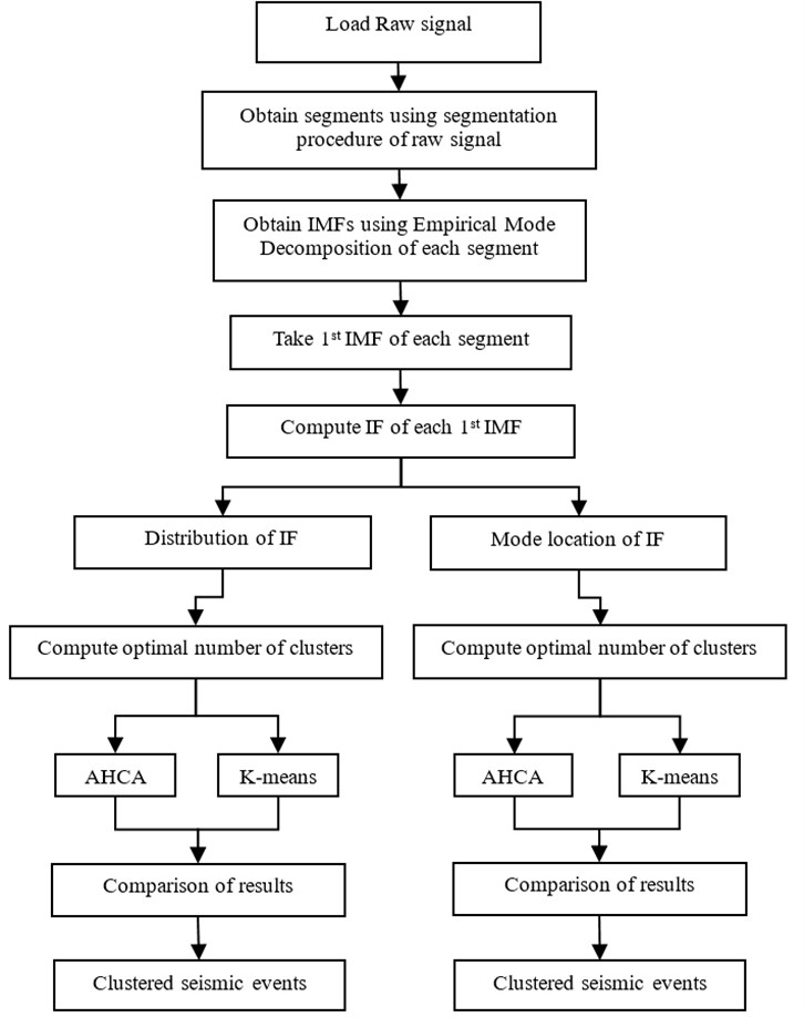
Fig. 1Diagram of signal analysis’ procedure
2.6. Silhouettes method
Clustering procedures require an a priori assumed number of clusters. So there is a need to estimate the optimal number of clusters in analyzed data. Visual analysis of clustering procedure results can be supported/dismissed by e.g. silhouettes [26]. Their construction is based on the concept of average dissimilarities between an object and other elements in clusters. One can construct a silhouette statistic, which for a fixed number of clusters assigns to th observation following value:
where is the average distance to cotenants in cluster where th case is allocated and is a distance to nearest neighboring cluster’s center. The final output of the silhouettes method is (silhouette coefficient) and this value is therefore interpreted according to Table 1. The value of the criterion varies from 0 to 1.
Average value of silhouettes over all data (Silhouette Coefficient, ) is a measure of how properly the clustering is performed. Table 1 represents interpretation of proposed by Kaufman and Rousseeuw [18].
The entire procedure of signal preparation before clustering is presented in (Fig. 1).
Table 1Subjective interpretation of the SC
Proposed interpretation | |
0.7 | A strong structure has been found |
0.5 0.7 | A reasonable structure has been found |
0.25 0.5 | The structure is weak and could be artificial; please try additional methods on this data set |
0.25 | No substantial structure has been found |
3. Application
Seismic vibration signals analyzed in this paper are acquired using a sensor independent to the commercial seismic system installed in the underground copper ore mine.
The sensor is a triaxial accelerometer mounted on the mining corridor roof using gypsum binder (Fig. 2).
Fig. 2The accelerometer located on the mining corridor roof
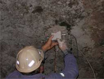
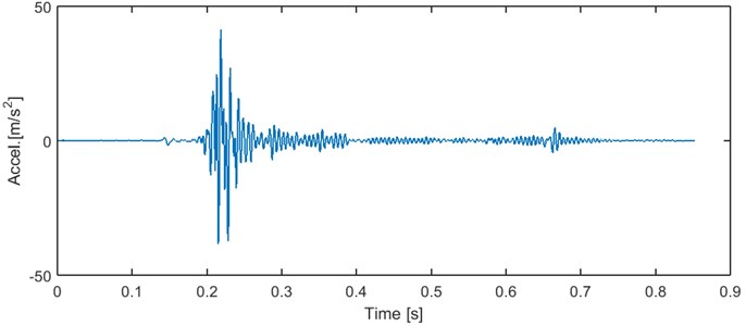
Range of sensor is 0.001 to 100 m/s2, frequency range is 0.5-400 Hz and sampling frequency is set to 1250 Hz. The distance between the sensor and the mining face was systematically rising (due to progress of mining works) from 20 m to 140 m. Signals’ noise level is relatively low, as it can be seen in Fig. 3.
3.1. Data preparation
In this paper we analyze 98 signals (segments) which are obtained from 51 seismic recordings.
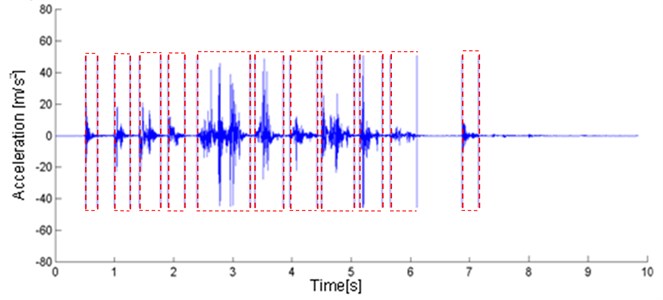
In Fig. 4 one can find an exemplary result of the segmentation procedure described in [19]. Trimming property is easy to notice. What also could be noted is that near 3 s there is a segment that consists of couple single events. When single excitations are overlapping, segmentation procedure may have difficulties in division.
Fig. 3Typical recording of a seismic signal (natural event)
After the segmentation single-event signals are subjected to EMD algorithm and, as it was mentioned, for each segment we compute instantaneous frequency of a first IMF.
Fig. 4Typical recording of a seismic signal (mining face blasting) with applied segmentation
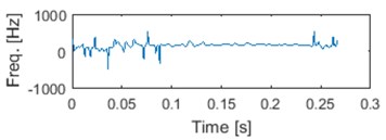
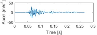
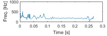
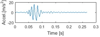
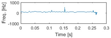
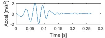
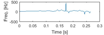
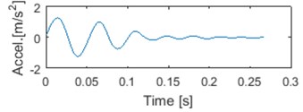
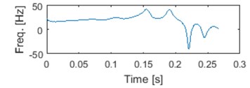
In Fig. 5. we can see an exemplary segment, first four IMFs and corresponding IFs. It can be noticed that IF of raw signal is meaningless, since negative frequencies can be noticed [15]. Also some negative values might be seen on IF of 4th IMF. It is due to possible imperfection of IF from IMF. There exist methods that can deal with that problem [27, 28]. However, we assume that problem of negative IMFs’ IF is in this case marginal and we haven’t considered it further yet.
Afterwards, 2 features are extracted from IFs, that were proposed by the Authors in [5].
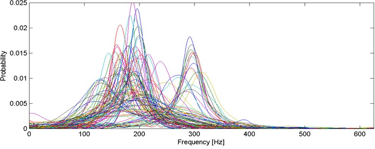
First of the discrimination features is a vector of probability density function values of the 1st IMF’s IF, derived from Rozenblatt-Parzen kernel density estimator with Gaussian kernel [22, 23], in fixed number of points (i.e. 512), located uniformly between 0 and 625 Hz (as the sampling frequency of gathered data is 1250 Hz). In Fig. 6, we present the segments’ first feature representations.
The second feature, which is specific condensation of the previous one, represents each seismic signal segment by its dominant frequency of 1st IMF’s IF. With such reduction we lose significant part of information, however it is simpler to decide whether two clusters shall be cotenants or not. In Fig. 7 we include values of 2nd feature presented on a histogram.
Fig. 5Typical seismic signal with 5 first IMFs and corresponding instantaneous frequencies
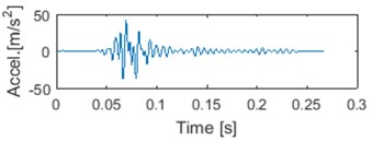
a) Signal
b) IF of signal
c) 1 IMF
d) IF of 1 IMF
e) 2 IMF
f) IF of 2 IMF
g) 3 IMF
h) IF of 3 IMF
i) 4 IMF
j) IF of 4 IMF
Fig. 6Probability density function estimators for all segments
3.2. Silhouette results
Each feature was analyzed by silhouettes in order to find optimal number of classes. The results are presented in a table below.
As it can be seen from Table 2, best results of for distribution of IF, are acquired with two-cluster division (for both clustering methods). for dominate over other options. All results may be interpreted as “reasonable structures” (Table 1). The differences between clustering methods for are not significant, i.e. each value of is between 0.5 and 0.7.
Fig. 7Histogram of 2nd feature values

Table 2SC results: IF’s distribution
Feature | Clustering | ||||||
Distribution of IF | AHCA | 0.6555 | 0.5501 | 0.5022 | 0.5208 | 0.5310 | 0.5253 |
-means | 0.6510 | 0.5246 | 0.5094 | 0.5389 | 0.5479 | 0.5743 |
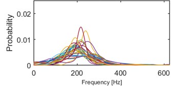
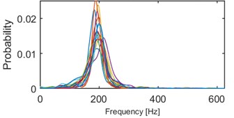
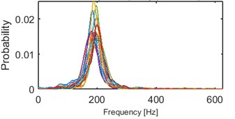
Fig. 8Results of IF density estimator – 98 segments grouped into 2 clusters by both algorithms
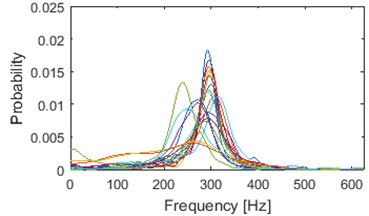
a)-means cluster 1/2
c) AHCA cluster 1/2
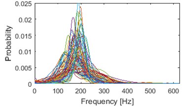
b)-means cluster 2/2
d) AHCA cluster 2/2
Illustration of clustering into 2 groups obtained using k-means and AHCA is presented in Fig. 8. Results of AHCA and k-means are mostly coinciding. First cluster (for both methods) possess dominant shape of densities: medium-dispersal with mode located around 300 Hz. Additionally, couple of visible outliers are located in this cluster, however their number is negligible (-means: 6, AHCA: 4). Cluster 1 (especially after AHCA) seems to be well build. However, cotenants in the 2nd cluster seems to be too much diversified in terms of dispersion and dominant frequency. It is possible that clustering with another number of groups would be much better in terms of visual inspection.
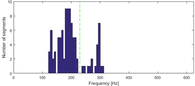
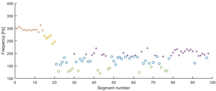
Table 3 shows that the second feature has as an optimal number of clusters. Results for all sets from to are evaluated as “strong structures” (Table 1). Number of clusters that was evaluated as the least is (-means) and (AHCA). On the other hand, in Fig. 9 one can notice several modes in distribution of the feature. Similar to method presented in [29], we divide the frequency axis in order to separate each significant mode.
In Fig. 9 results of k-means and AHCA clustering are contained. Segments which are on the left side of the line have been allocated in the first cluster, and these on the right side – in the second one. The line does not indicate any specific frequency. Both of the methods separated the segments into 2 groups in the same way. Although, 4 clear modes can be noticed in the histogram. Moreover, 6 segments with mode located between 230 and 280 Hz could even build another group.
This leads us to believe that visual-best results may not be consistent with that obtained from the automatic algorithm.
Table 3SC results: location of the mode
Feature | Clustering | ||||||
Location of the mode | AHCA | 0.8694 | 0.8051 | 0.7451 | 0.7426 | 0.7689 | 0.7933 |
-means | 0.8694 | 0.8090 | 0.7305 | 0.7896 | 0.7974 | 0.7943 |
Fig. 9Location of the mode – 98 segments partitioned into 2 clusters by k-means and AHCA
3.3. Best visual results
Recall that the silhouette method indicated that 2 is the optimal number of clusters for both instantaneous frequency features. However, visual inspection of these results (Fig. 8, Fig. 9) pointed out that the obtained clusters consist of segments that differ significantly in terms of dominant mode and density of instantaneous frequency. Thus, an attempt to find the number of clusters which would better fulfill the main assumptions of good clustering (similar cotenants and different neighboring clusters) has been made.
By empirical tests we decided, that 5 is the best number of classes for density of IF. Lower quantity makes cotenants too different, and the larger make neighboring clusters too similar.
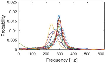
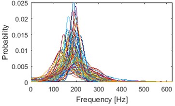
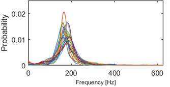
Clustering results of AHCA (Fig. 11) seems to be consistent with those derived by the k-means (Fig. 10). Such phenomenon indicates high robustness of a discrimination feature. As it can be seen, the algorithm distributed the segments with respect to theirs IF distribution and dominant frequency value. Instantaneous frequencies concentrate in one of 4 different modes 140 Hz, 170 Hz, 200 Hz (2 groups) and 300 Hz. They manifest different dispersions within the clusters. First set (140 Hz, 5/5 in Fig. 10, 1/5 in Fig. 11) has the highest dispersion, also in couple of its segments multimodal feature can be seen. Set which has the 2nd lowest dispersion (200 Hz, 3/5 in Fig. 10, 2/5 in Fig. 11), shares modal frequency with the set whose dispersion is largest (200 Hz, 4/5 in Fig. 10, 4/5 in Fig. 11). 3rd (170 Hz, 2/5 in Fig. 10, 3/5 in Fig. 11) and 5th (300 Hz, 1/5 in Fig. 10, 5/5 in Fig. 11) clusters have similar dispersions, but different modes.
Fig. 10Results of clustering using IF density estimator – 98 segments partitioned into 5 clusters, k-means
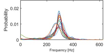
a) Probability of frequency (cluster 1/5)
b) Probability of frequency (cluster 2/5)
c) Probability of frequency (cluster 3/5)
d) Probability of frequency (cluster 4/5)
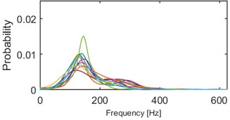
e) Probability of frequency (cluster 5/5)
Fig. 11Results of clustering using IF density estimator – 98 segments partitioned into 5 clusters, AHCA
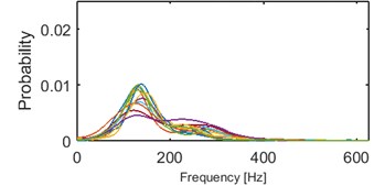
a) Probability of frequency (cluster 1/5)
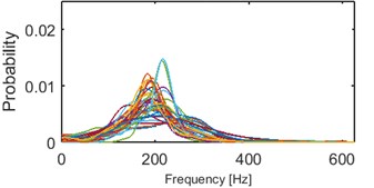
b) Probability of frequency (cluster 2/5)
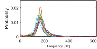
c) Probability of frequency (cluster 3/5)
d) Probability of frequency (cluster 4/5)
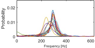
e) Probability of frequency (cluster 5/5)
One can notice couple outliers (Fig. 10 cluster 1/5 and 3/5, Fig. 11 cluster 2/5 and 5/5). They correspond to 6 segments with mode located between 230 and 280 Hz in Fig. 9. Thus considering them as outliers in terms of this feature may guide to repeat consideration for the second discrimination feature.
The AHCA four-cluster results seems to be reliable (Fig. 12). The clusters are similar to those obtained from first feature. The clusters are concentrated in 140 Hz, 170 Hz, 200 Hz, and 300 Hz (outliers are allocated in this set). Two groups of segments with mode located around 200 Hz from previous discrimination feature are now merged into one set.
Fig. 12Results of clustering using mode location – 98 segments partitioned into 4 clusters, AHCA
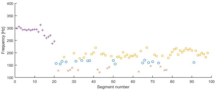
However, when -means is applied couple of times with 4 as a number of clusters it can be noticed, that in many cases outliers form a separate set (see Fig. 13). Thus, there must be such a cluster that contains segments with significantly different modes (here, clusters with modes at 140 Hz and 170 Hz), which seems to be an inappropriate result (due to analysis of Fig. 9). Thus, we consider 5 clusters to improve clustering results.
The results of AHCA clustering into 5 groups divide the cluster with modes centered around 300 Hz into 2 clusters: segments with dominant frequency around 300 Hz and 6 outliers mentioned previously.
Fig. 13Results of clustering using mode location – 98 segments partitioned into 4 clusters, k-means
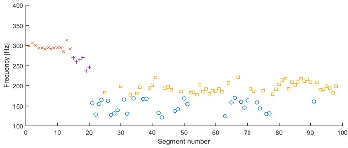
In Fig. 14 we can see -means clustering. The segments with modes at 170 Hz are slightly mixing with the 200 Hz segments. The algorithm tends to return a bit random assignment especially for outliers and segments represented by modes between 200 and 170 Hz. However, the general results are satisfying, since -means does not merge all of the segments with modes between 170 and 200 Hz into one cluster.
The fact that 2 different clustering methods return us similar (or even the same) results proves reliability and robustness of the considered features.
Fig. 14Second feature under the k-means, 5 clusters
4. Conclusions
In this paper we analyzed two different discrimination features which deal with the problem of analyzing similarities of seismic signals. We used silhouette-based method which was expected to answer the question, what is optimal number of clusters which considered features divide the segments. Unfortunately, results obtained from this method seems not to be consistent with requirements regarding reliable clustering. The visual analysis demonstrated another number of clusters as trustworthy. We hope to find in the future work another algorithms evaluating the optimal number of clusters consistent with visual analysis. Further work could be also related to improvement of each step of the method that returns the instantaneous frequency, e.g. the normalized Hilbert transform [27].
However, empirical tests proved that both features based on the instantaneous frequency may be successfully used in seismic signals discrimination, as the cotenants are similar, and neighboring clusters differs significantly. This fulfills the imposed expectations.
References
-
Malovichko D. Discrimination of blasts in mine seismology. Proceedings of the Deep Mining, Australian Centre for Geomechanics, Perth, Australia, 2012.
-
Gibowicz S. J., Kijko A. An Introduction to Mining Seismology. Academic Press, San Diego, 1994.
-
Ma J., Zhao G., Dong L., Chen G., Zhang C. A comparison of mine seismic discriminators based on features of source parameters to waveform characteristics. Shock and Vibration, 2015.
-
Ouyang Z., Qi Q., Zhao S., Wu B., Zhang N. The mechanism and application of deep-hole precracking blasting on rockburst prevention. Shock and Vibration, 2015.
-
Sokolowski J., Obuchowski J., Madziarz M., Wylomanska A., Zimroz R. Seismic signals discrimination based on instantaneous frequency. Vibroengineering Procedia, Vol. 6, 2015, p. 200-205.
-
Yan R., Gao R. X. Hilbert-Huang transform-based vibration signal analysis for machine health monitoring. IEEE Transactions on Instrumentation and Measurement, Vol. 55, Issue 6, 2006, p. 2320-2329.
-
Yinfeng D., Yingmin L., Mingkui X., Ming L. Analysis of earthquake ground motions using an improved Hilbert-Huang transform. Soil Dynamics and Earthquake Engineering, Vol. 28, Issue 1, 2008, p. 7-19.
-
Huang N. E., Wu M.-L., Qu W., Long S. R., Shen S. S. P. Applications of Hilbert-Huang transform to non-stationary financial time series analysis. Applied Stochastic Models in Business and Industry, Vol. 16, Issue 3, 2003, p. 245-268.
-
Huang N. E., Shen Z., Long S. R., Wu M. C., Shih H. H., Zheng, Yen N., Chao Tung C., Liu H. H. The empirical mode decomposition and the Hilbert spectrum for nonlinear and non-stationary time series analyses. Proceedings of the Royal Society of London Series A-Mathematical Physical and Engineering Sciences, Vol. 454, 1998, p. 903-995.
-
Flandrin P., Rilling G., Goncalves P. Empirical mode decomposition as a filter bank. Signal Processing Letters, Vol. 11, Issue 2, 2004, p. 112-114.
-
Dybala J., Zimroz R. Rolling bearing diagnosing method based on empirical mode decomposition of machine vibration signal. Applied Acoustics, Vol. 77, 2014, p. 195-203.
-
Liu B., Riemenschneider S., Xu Y. Gearbox fault diagnosis using empirical mode decomposition and Hilbert spectrum. Mechanical Systems and Signal Processing, Vol. 20, Issue 3, 2006, p. 718-734.
-
Battista B. M., Knapp C., McGee T., Goebel V. Application of the empirical mode decomposition and Hilbert-Huang transform to seismic reflection data. Geophysics, Vol. 72, Issue 2, 2007, p. 29-37.
-
Loh C. H., Wu T. C., Huang N. E. Application of the empirical mode Decomposition-Hilbert spectrum method to identify near-fault ground-motion characteristics and structural responses. Bulletin of the Seismological Society of America, Vol. 91, Issue 5, 2001, p. 1339-1357.
-
Boashash B. Estimating and interpreting the instantaneous frequency of a signal – part 1: fundamentals. Proceedings of the IEEE, Vol. 80, Issue 4, 1992, p. 520-538.
-
Macqueen J., et al. Some methods for classification and analysis of multivariate observations. Proceedings of the fifth Berkeley Symposium on Mathematical Statistics and Probability, Vol. 1, Issue 14, 1967, p. 281-297.
-
Lloyd S. P. Least squares quantization in PCM. IEEE Transactions on Information Theory, Vol. 28, Issue 2, 1982, p. 129-137.
-
Kaufman L., Rousseeuw P. J. Finding Groups in Data: An Introduction to Cluster Analysis. First Edition, Wiley-Interscience, New Jerseym 2005.
-
Zimroz R., Madziarz M., Żak G., Wyłomańska A., Obuchowski J. Seismic signal segmentation procedure using time-frequency decomposition and statistical modelling. Journal of Vibroengineering, Vol. 17, Issue 6, 2015, p. 3111-3121.
-
Gabor D. Theory of communication. Part 1: the analysis of information. Journal of the Institution of Electrical Engineers – Orat III: Radio and Communication Engineering, Vol. 93, Issue 26, 1946, p. 429-441.
-
Rilling G., Flandrin P., Goncalves P. On empirical mode decomposition and its algorithms. IEEE – EURASIP Workshop on Nonlinear Signal and Image Processing, Vol. 3, 2003, p. 8-11.
-
Rosenblatt M. Remarks on some nonparametric estimates of a density function. The Annals of Mathematical Statistics, Vol. 27, Issue 3, 1956, p. 832-837.
-
Parzen E. On estimation of a probability density function and mode. The Annals of Mathematical Statistics, Vol. 33, Issue 3, 1962, p. 1065-1076.
-
David A., Vassilvitskii S. K-means++: the advantages of careful seeding. Proceedings of the Eighteenth Annual ACM-SIAM Symposium on Discrete Algorithms, Society for Industrial and Applied Mathematics, Philadelphia, 2007.
-
Ward J. H. Jr. Ward’s hierarchical agglomerative clustering method: which algorithms implement Ward’s criterion. Journal of Classification, Vol. 31, Issue 3, 2014, p. 274-295.
-
Rousseeuw P. J. Silhouettes: a graphical aid to the interpretation and validation of cluster analysis. Journal of Computational and Applied Mathematics, Vol. 20, 1987, p. 53-65.
-
Huang N. E., Long S. R. Normalized Hilbert Transform and Instantaneous Frequency. NASA Patent Pending GSC, Vol. 14, 2003, p. 673-680.
-
Huang N. E., Shen S. S. Hilbert-Huang Transform and Its Applications. Second Edition, World Scientific Publishing Co. Pte. Ltd., Singapore, 2013.
-
Makowski R., Zimroz R. Parametric time-frequency map and its processing for local damage detection in rotating machinery. Key Engineering Materials, Vol. 588, 2014, p. 214-222.
Cited by
About this article

Jakub Sokołowski implemented algorithms and prepared the paper. Jakub Obuchowski is the author of a concept to analyze seismic signals’ similarities via instantaneous frequency. Maciej Madziarz carried out the data acquisition experiment and interpreted the recordings. Agnieszka Wyłomańska suggested seismic recordings segmentation method and tested reliability of the results. Radosław Zimroz provided the required signal processing, mining knowledge and suggested methodology.
