Fault diagnosis of rolling bearing based on improved CEEMDAN and distance evaluation technique

Ding, Feng; Li, Xiang; Qu, Jinxiu

doi:10.21595/jve.2016.17398

Journal of Vibroengineering

Browse Journal

Submit article

Published: 15 February 2017

Check for updates

Fault diagnosis of rolling bearing based on improved CEEMDAN and distance evaluation technique

Feng Ding¹

Xiang Li²

Jinxiu Qu³

^{1, 2, 3}Department of Mechanical and Electronic Engineering, Xi’an Technological University, Xi’an, China

Corresponding Author:

Feng Ding

Cite the article Download PDF

Downloads 1828

WoS Core Citations 10

CrossRef Citations 13

Abstract

In order to accurately identify the fault conditions of rolling bearing, this paper presents a fault diagnosis method based on improved complete ensemble empirical mode decomposition with adaptive noise (CEEMDAN) and distance evaluation technique. In this method, to effectively extract potential fault-related information, vibration signals of rolling bearing in different fault conditions are decomposed into a set of intrinsic mode functions (IMFs) through improved CEEMDAN. The first eight IMFs containing most fault information are selected for extracting fault features. The original feature set is obtained including energy values, singular values and envelope sample entropy values. Then distance evaluation technique is implemented for selecting sensitive feature set and discarding irrelevant or redundant features. Subsequently, the sensitive feature set is fed into support vector machine (SVM) for automatically identifying rolling bearing fault conditions. The simulation results demonstrate that improved CEEMDAN is able to solve the problem of mode mixing and achieve a numerically negligible reconstruction error. Meanwhile experimental consequences indicate that the proposed method can acquire higher identification accuracy, as well as reduce the classifier computational burden.

1. Introduction

As one of the most important part of rotating machinery, rolling bearing is extremely significant for ensuring reliable operation of the whole mechanical system. In the long-time running process, damage of rolling bearing components will inevitably take place. It will lead to some kinds of faults and severely influence the operation condition of machine [1]. Therefore, it is essential to monitor the condition of rolling bearing and detect faults as early as possible [2].

In recent years, rolling bearing fault diagnosis has become the research focus and received considerable attention from many scholars around the world. At present, the primary means of fault diagnosis is to obtain underlying fault-related information via processing vibration signals [3, 4]. However, rolling bearing vibration signals are usually nonstationary and nonlinear with a large amount of background noise. It is particularly difficult to achieve useful fault information. Thus, an effective signal processing method is demanded urgently.

Empirical mode decomposition (EMD) is an adaptive method which is suitable for multiscale decomposition and time-frequency analysis of nonlinear and nonstationary signals. More specifically, it can decompose signals into a set of intrinsic mode functions (IMFs) under the local characteristic time scales [5]. The IMFs are amplitude and frequency modulated components and an ultimate monotonic residue signal is obtained. EMD has been successfully utilized in different fields due to its attractive advantage of dyadic filter bank and achieved ideal effects [6, 7]. Nevertheless, there are still some problems existing in the process of EMD, and one of the most serious drawbacks is the mode mixing phenomenon. It means that oscillations of quite disparate scales are produced in one mode or oscillations with similar scales appear in different modes. In order to alleviate the mode mixing or aliasing, a noise assisted signal decomposition method called ensemble EMD (EEMD) is applied in some situations [8, 9]. By using EEMD, different scale oscillations in the signals can be automatically projected onto the appropriate reference framework, which is established by white noise based on the property of uniform distribution of spectrum. However, the influence of added noise on the decomposition effect is not completely offset through limited averaging processing. In a word, residue white noise still exists in the reconstructed components. The computation quantity is larger while reconstruction error can be reduced by increasing the number of ensemble trials.

To settle the problem that the reconstruction signals are contaminated by residue noise, complementary EEMD (CEEMD) is presented via adding white noise in pairs with opposite signs to the targeted signals [10, 11]. Although it outperforms EEMD in eliminating the effect of remaining noise, it is still indispensable that a great number of ensemble trials need to be carried out. Moreover, the number of generated IMFs is different since diverse realizations of signal plus noise. It leads to the problem that the final averaging calculation is difficult to implement. The inappropriate parameters including the amplitude of white noise and the number of ensemble trials can also result in the generation of spurious modes. For the purpose of overcoming these situations, Torres et al. [12] propose an improved algorithm called complete EEMD with adaptive noise (CEEMDAN). It provides a new approach to reconstruct original signals with a numerically negligible error and lower computational consumption. In each stage of the decomposition of this method, an adaptive white noise is added and the unique residue signal is calculated to obtain the individual modes. It has been proven to be effective in areas such as biomedical engineering [12, 13] and energy economics [14].

Indeed, CEEMDAN can avoid the mode mixing phenomenon and its decomposition process is complete. Yet, some minor aspects such as the presence of little residue noise in IMFs and the emergence of false modes still deserve to be ameliorated. Colominas et al. [15] put forward improvements on CEEMDAN to obtain IMFs with less residue noise and more abundant physical significance. The advantages of the new method have been demonstrated in analysis of artificial signals and actual biomedical signals.

In addition, eigenvalue analysis has been performed availably in the study of vibration behaviors of gradient elastic micro beams and carbon nanotubes [16, 17]. By eigenvalue or modal analysis, the vibration frequencies of mechanical systems can be controlled and some problems which are caused by resonance can also be prevented. Normally, eigenvalues are closely related to the conditions of systems. Hence, it is necessary to extract appropriate fault features for accurately identifying variable rolling bearing fault types. In this paper, vibration signals of rolling bearing are decomposed through improved CEEMDAN. To reveal rolling bearing fault conditions from multiple aspects, the original feature set is obtained including energy values, singular values and envelope sample entropy values. Afterwards, distance evaluation technique is employed for selecting sensitive feature set and discarding irrelevant or redundant features. In the end, the sensitive feature set is as the input of support vector machine (SVM) to automatically identify fault conditions of rolling bearing.

The remaining parts of this paper are organized as follows. In Section 2, theoretical knowledge of improved CEEMDAN is briefly described, and the simulation experiment is conducted to confirm the feasibility and effectiveness of improved CEEMDAN in eliminating mode mixing and reducing reconstruction error. Feature extraction and sensitive features selection based on distance evaluation technique are presented in Section 3. The whole procedure of rolling bearing fault diagnosis is provided in Section 4. In Section 5, the proposed method of this paper is employed in the rolling bearing fault diagnosis. Last but not least, conclusions or summaries are drawn in Section 6.

2. Improved CEEMDAN

2.1. Algorithm of improved CEEMDAN

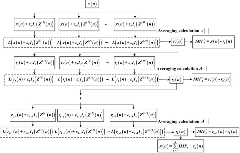
It has been certified in literature [12] that CEEMDAN outperforms EEMD in removing the residue noise of modes and exactly reconstructing original signals. In EEMD algorithm, each realization of signal plus white noise is decomposed independently from the others and the decomposition of each realization produces a residue. Hence, the final modes are obtained by averaging processing, and it leads to the issue that the existence of residue noise in IMFs. In the method of CEEMDAN, the first IMF is achieved in the same way as EEMD. However, during the procedure of obtaining other modes, only a residue is produced in each stage of decomposition. Let $r_{k} (n)$ be the $k$ th residue and $I_{k} (\cdot)$ is defined as the operator which produces the $k$ th IMF via EMD. Let $Z^{(m)} (n)$ ( $m =$ 1, 2,…, $M$ ) represent the $m$ th realization of zero mean Gaussian white noise and $ε_{k}$ is the desired signal-to-noise ratio (SNR) between the added noise and the residue signal.

The $k$ th residue and the $(k + 1)$ th IMF are respectively expressed as:

1

r_{k} (n) = r_{k - 1} (n) - I M F_{k}^{'} (n),

2

I M F_{k + 1}^{'} (n) = \frac{1}{M} \sum_{m = 1}^{M} I_{1} (r_{k} (n) + ε_{k} I_{k} (Z^{(m)} (n))) .

The decomposition process continues until the obtained residue satisfies the iterative stopping criterion, that is the residue has at most two extrema. Despite of that, there are some minor aspects which still deserve to be further ameliorated. The issues which should be addressed mainly include two parts: 1) the existence of little residue noise in IMFs; 2) the appearance of spurious modes.

Taking into account the above shortcomings, improved CEEMDAN is presented and demonstrated to be more effective. Here, $L (\cdot)$ is defined as the operator which can calculate the local mean of signals. Except that, $A |\cdot|$ denotes the averaging calculating operation of different realizations and $x (n)$ is the original signal. The algorithm of improved CEEMDAN is described as follows, and the specific flowchart is shown in Fig. 1.

Step 1: Calculate the first IMF of $M$ white noise realizations, respectively. Then the final local mean is obtained, and the first residue can be presented as:

3

r_{1} (n) = A |L (x (n) + ε_{0} I_{1} (Z^{(m)} (n)))| .

Step 2: The first IMF is calculated as:

4

I M F_{1}^{'} = x (n) - r_{1} (n) .

Step 3: Compute the second IMF of $M$ white noise realizations, and estimate the average local mean of all ensemble trials to obtain the second residue:

5

r_{2} (n) = A |L (r_{1} (n) + ε_{1} I_{2} (Z^{(m)} (n)))| .

Step 4: The second IMF are extracted as follows:

6

I M F_{2}^{'} = r_{1} (n) - r_{2} (n) = r_{1} (n) - A |L (r_{1} (n) + ε_{1} I_{2} (Z^{(m)} (n)))| .

Step 5: Let $k$ from 3 to $K$ , evaluate the $k$ th residue and the $k$ th IMF individually:

7

r_{k} (n) = A |L (r_{k - 1} (n) + ε_{k - 1} I_{k} (Z^{(m)} (n)))|,

8

I M F_{k}^{'} = r_{k - 1} (n) - r_{k} (n) .

Step 6: Continue the above decomposition until the acquired residue $r (n)$ is no longer admitted to be decomposed. In the end, the original signal $x (n)$ can be expressed as:

9

x (n) = \sum_{k = 1}^{K} I M F_{k}^{'} + r (n) .

Fig. 1The algorithm flowchart of improved CEEMDAN

2.2. Evaluation and comparison of EEMD, CEEMDAN and improved CEEMDAN

EEMD is a noise assisted method which can solve the problem of mode mixing in the conventional EMD. However, the premise of this conclusion is that a large number of noise ensemble trials are performed, and it greatly increases the time complexity of the algorithm. Compared with EEMD, CEEMDAN can eliminate the phenomenon of mode mixing by the finite number of noise ensemble averaging operation. Furthermore, the numerical reconstruction error is nearly negligible, and it overcomes the drawbacks of EEMD in low efficiency and incompleteness. The aforementioned improved CEEMDAN method can further remove the minor white noise in the modes, and over decomposition problem can also be settled.

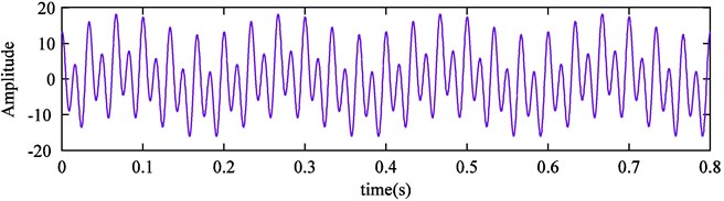
EEMD, CEEMDAN and improved CEEMDAN are used separately to decompose the simulation signal. Then the IMFs components and the error of reconstruction signal are analyzed to verify above conclusions. In the course of decomposition, the number of ensemble trials is set as 100 and the noise standard deviation is 0.2 (the same two parameters are set when they are used in the full text). The simulation signal $x$ is consisted of the following three parts:

10

\{\begin{array}{l} x 1 = 10 s i n (2 π \times 60 t + \frac{π}{2}), \\ x 2 = 6 s i n (2 π \times 30 t + \frac{π}{3}), \\ x 3 = 3 s i n (2 π \times 5 t - \frac{π}{4}) . \end{array}

Gaussian white noise is added into the simulation signal, and the SNR of obtained signal is 36 db. The sampling frequency is 3.6 kHz and the sampling time is 0.8 second. The time domain waveform of simulation signal is shown in Fig. 2.

Fig. 2Time domain waveform of simulation signal

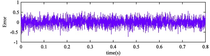
Firstly, the signal is decomposed by EEMD, and the results are shown in Fig. 3. It can be seen that ten modes are produced and IMF4, IMF5, IMF6 correspond with $x_{1}$ , $x_{2}$ , $x_{3}$ respectively. Yet, obvious oscillations with other scales exist in the IMF3, and that is the mode mixing phenomenon. It indicates that EEMD is not able to achieve good decomposition effect in the case of less ensemble trials. Furthermore, the error between reconstruction signal and original signal is presented in Fig. 4. And we can find that the EEMD is not complete and larger error occurs in this case.

Fig. 3EEMD results of simulation signal

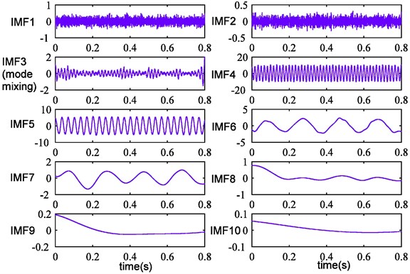
Fig. 4EEMD reconstruction error of simulation signal

After that, the simulation signal is processed by CEEMDAN. From the Fig. 5, we can see that twelve IMFs are generated and IMF6, IMF7, IMF9 correspond with the real three components. Compared with EEMD, the mode mixing problem is restrained, but IMF8 which is contaminated by little noise is obtained simultaneously. The Fig. 6 describes the result of reconstruction error, and it can be observed that the magnitude order of error declines significantly.

Fig. 5CEEMDAN results of simulation signal

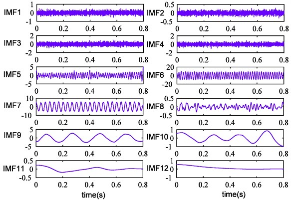
Fig. 6CEEMDAN reconstruction error of simulation signal

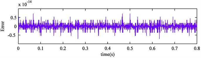
Fig. 7Improved CEEMDAN results of simulation signal

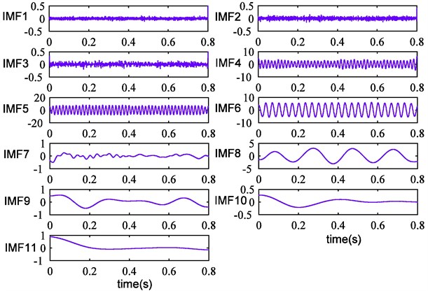
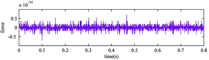
Improved CEEMDAN is utilized in the simulation signal processing. The decomposition outcome is exhibited in Fig. 7. It can be seen that ten IMFs and a final residue are obtained. Further analysis shows that IMF5, IMF6, IMF8 are the actual components of the simulation signal. Compared with Fig. 5, fluctuation of obtained modes is more stable and the mode mixing problem is completely eliminated. Moreover, the remaining noise in IMF7 is removed and one high-frequency spurious mode is also eliminated successfully. The reconstruction error is displayed in Fig. 8, we can discover that the error is reduced further. Therefore, it can demonstrate that improved CEEMDAN is effective and complete, and the above conclusions can be confirmed strongly.

Fig. 8Improved CEEMDAN reconstruction error of simulation signal

3. Feature extraction and selection

3.1. Feature extraction based on improved CEEMDAN

Considering the advantages of improved CEEMDAN, it is applied to process the vibration signals of rolling bearing. A set of components with different scales from high to low frequencies are obtained. Generally, the first eight IMFs contain plentiful physical information. Hence, the feature indicators which are extracted from these IMFs are able to reflect the running conditions of rolling bearing. In this paper, three kinds of features are calculated to provide valuable information for the following fault diagnosis.

3.1.1. Energy feature

When rolling bearing is in variable fault conditions, the intrinsic characteristic frequencies are different from each other. Furthermore, improved CEEMDAN can decompose original signals into the corresponding frequency-band signals. It leads to the result that the energy distribution of different frequency-band signals changes with the conditions of rolling bearing. In another word, the uncertainty of signals energy distribution is different. Naturally, the feature vector which is composed of the energy of the first eight IMFs can distinguish different fault types. Therefore, the energy feature vector $E = \{E_{1}, E_{2}, \dots, E_{8}\}$ is achieved in this paper. The energy values are acquired through the following Eq. (11):

11

E_{j} = \sum_{i = 1}^{n} {[x (i)]}^{2},

where $x (i)$ denotes the amplitude of IMFs discrete points, $i =$ 1, 2,…, $n$ is the number of discrete points of IMFs.

3.1.2. Singular value feature

Singular value decomposition (SVD) is an orthogonal matrix decomposition method, and singular values represent the inherent characteristics of matrix. Admittedly, they have excellent stability, and almost remain unchanged while minor changes occur in matrix [18, 19]. As a precise data-driven processing method, SVD is widely employed in many investigation fields including feature extraction and signal processing.

The matrix which is formed of the first eight IMFs contains most useful condition information. However, the IMFs are usually so complicated that they cannot immediately serve as the input feature vectors of the classifier. In order to deal with the deficiency, SVD is introduced to extract the main features and compress the scale of the IMFs. Specifically, the IMFs matrix elements of diverse fault conditions differ from each other significantly, as well as there are only slight differences in the IMFs matrix of different samples from the same fault type. Thus, we can draw the conclusion that the singular values of IMFs matrix in different fault conditions can be clearly discriminated. It satisfies the requirement of fault identification. Moreover, the robustness of fault feature vectors is also enhanced.

According to the analysis above, singular values $S = \{S_{1}, S_{2}, \dots, S_{8}\}$ of IMFs matrix are selected to serve as fault features.

3.1.3. Envelope sample entropy feature

It produces a series of pulse forces when rolling bearing damage site contacts with its element surface, and the frequency of pulse force is the so-called fault feature frequency. In the meantime, the inherent vibration frequency of rolling bearing is much higher than the feature frequency. Thus, the main fault information is hidden in the modulation signals. The fault-related features can be obtained from the envelope demodulation signals by Hilbert transform to IMFs [20].

On the other hand, there are several nonlinear parameter estimation methods such as permutation entropy [21], sample entropy [22], etc. The methodology of sample entropy supplies an alternative to excavate underlying condition-related information. It is a kind of means for estimating sequence complexity. In addition, sample entropy is independent to the signal length and has fine stability. Hence, we extract the sample entropy of IMFs envelope signals $Y = {Y_{1}, Y_{2}, \dots, Y_{8}}$ as feature indicators.

Now, the original feature set containing twenty-four features is achieved, and the feature vector is constructed as $F V = {E_{1}, E_{2}, \dots, E_{8}, S_{1}, S_{2}, \dots, S_{8}, Y_{1}, Y_{2}, \dots, Y_{8}}$ .

3.2. Sensitive feature selection based on distance evaluation technique

The original feature set contains not only sensitive features, but also irrelevant or redundant features which may conflict with each other. The sensitive features include dominant condition-related information, and other uncorrelated features should be discarded for enhancing computational efficiency of the classifier. Besides, curse of dimensionality can be avoided.

The principle of selecting sensitive features is the ability to distinguish samples of different fault types. In practical, there are many sensitive feature selection methods which have been employed in actual situations, such as non-negation sparse principal component analysis (NSPCA) [23], neighborhood rough set (NRS) [24, 25], and distance evaluation technique [26, 27], etc. In view of the simplicity and reliability of distance evaluation technique, it is utilized to select sensitive features from the original feature set. Furthermore, it can greatly save the calculation time cost of the classifier.

The evaluation factor is defined as the ratio between the average distance of different and same condition samples. Larger evaluation factor means that the feature is more suitable for separating fault conditions, and identification effect of the classifier is better. The detailed algorithm is described as follows:

Assume the feature set which includes all kinds of rolling bearing fault conditions is:

12

\{f_{c, b, w}, c = 1,2, \dots, C; b = 1,2, \dots, B_{c}; w = 1,2, \dots, W\},

where $f_{c, b, w}$ represents the $w$ th eigenvalue of the $b$ th sample in the $c$ th condition, and $B_{c}$ denotes the sample number of the $c$ th condition. There is a total of $C \times B_{c}$ samples. $W$ is the number of features in each sample, and $C \times B_{c} \times W$ is the number of all features.

Step 1: Calculate the average inner-class distance of the same condition samples:

13

d_{c, w} = \frac{1}{B_{c} (B_{c} - 1)} \sum_{s, t = 1}^{B_{c}} |f_{c, s, w} - f_{c, t, w}|, s, t = 1,2, \dots, B_{c}, s \neq t,

then achieve the average inner-class distance of all $C$ conditions:

14

D_{w}^{(a)} = \frac{1}{C} \sum_{c = 1}^{C} d_{c, w} .

Step 2: Compute the average eigenvalue of all samples in the $c$ th condition:

15

q_{c, w} = \frac{1}{B_{c}} \sum_{b = 1}^{B_{c}} f_{c, b, w},

then average distance between different condition samples can be expressed as follows:

16

D_{w}^{(v)} = \frac{1}{C (C - 1)} \sum_{e, h = 1}^{C} |q_{h, w} - q_{e, w}|, e, h = 1,2, \dots, C, e \neq h .

Step 3: Define and calculate the evaluation factor $α_{w}$ as follows:

17

α_{w} = \frac{D_{w}^{(v)}}{D_{w}^{(a)}} .

After that, the evaluation factors of all features are sorted from large to small. Starting from the most sensitive feature, the feature sets are composed by adding the number of features one by one. Then the sensitive feature sets are fed into the classifier for training and testing. Eventually, the most superior sensitive feature set is obtained, in which the number of features is the fewest and identification performance of the classifier is the most ideal.

4. The procedure of rolling bearing fault diagnosis

The detailed process of rolling bearing fault diagnosis is presented as follows: 1) vibration signals are decomposed into a set of IMFs by applying improved CEEMDAN, and the first eight IMFs are selected for extracting fault features; 2) the original feature set is obtained including energy values, singular values and envelope sample entropy values; 3) sensitive feature set is selected through distance evaluation technique; 4) due to the advantages in high accuracy and great generalization of SVM, the sensitive feature set of training sample is fed into SVM [28, 29]. Besides, genetic algorithm (GA) is an effective tool in global optimization. It is utilized to optimize SVM parameters for enhancing identification accuracy; 5) the testing sample is as the input of the trained SVM to automatically identify fault conditions of rolling bearing. The fault diagnosis model is exhibited in Fig. 9.

5. Experiment verification

5.1. Signal processing and feature extraction

The experiment data which is provided by the Bearing Data Center of Case Western Reserve University is investigated in this section. The sampling frequency of vibration signals is 12 kHz and the rotating speed of shaft is 1797 r/min. The data set includes 290 samples with ten kinds of fault conditions and each sample contains 4096 data points. The specific data set is exhibited in Table 1.

Fig. 9The flowchart of rolling bearing fault diagnosis

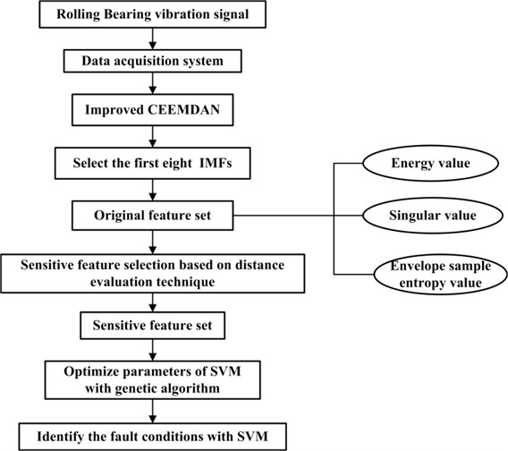
Table 1The specific description of data set

Fault type	Defect size (mm)	Number of training sample	Number of testing sample	Label
Inner race 1	0.1778	10	19	1
Inner race 2	0.3556	10	19	2
Inner race 3	0.5334	10	19	3
Outer race 1	0.1778	10	19	4
Outer race 2	0.3556	10	19	5
Outer race 3	0.5334	10	19	6
Normal	0	10	19	7
Rolling element 1	0.1778	10	19	8
Rolling element 2	0.3556	10	19	9
Rolling element 3	0.5334	10	19	10

Firstly, vibration signal of each sample is processed by improved CEEMDAN. The Fig. 10 shows the time domain waveform of rolling bearing outer race fault signal, and the defect size is 0.1778 mm. The first eight IMFs are presented in Fig. 11.

Fig. 10The time domain waveform of rolling bearing outer race fault signal

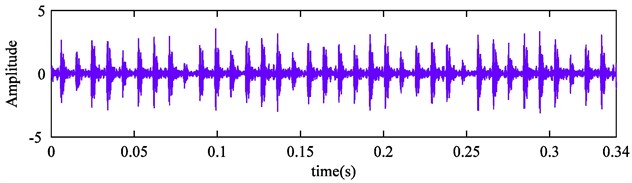
Fig. 11The first eight IMFs of rolling bearing outer race fault signal by improved CEEMDAN

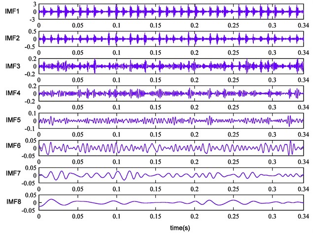
Fig. 12Energy values of the ten kinds of fault conditions

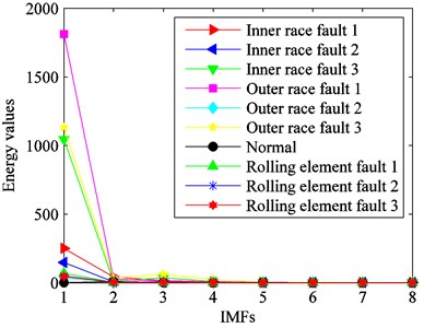
Fig. 13Singular values of the ten kinds of fault conditions

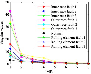
Fig. 14Envelope sample entropy values of the ten kinds of fault conditions

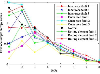
In the next step, the first eight IMFs are selected for calculating the energy values, singular values and envelope sample entropy values. The original feature set is obtained. In order to clearly reflect the sensitivity of features for identifying rolling bearing fault conditions, eigenvalues of various fault types are described in Fig. 12, Fig. 13 and Fig. 14. From these figures, we can see that eigenvalues of the first four IMFs can preferably distinguish the ten kinds of fault types. It indicates that some features are irrelevant or redundant and should be removed from the original feature set. Therefore, it is essential to select sensitive feature set for enhancing computational efficiency of classifier.

5.2. Sensitive feature selection

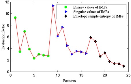
Distance evaluation technique is employed for selecting sensitive feature set. The evaluation factors of the twenty-four features are shown in Fig. 15. It can be found that evaluation factors of the first four IMFs are larger than others. It means that they are more sensitive for identifying rolling bearing fault conditions. Moreover, it is identical with the above theoretical analysis.

Fig. 15Feature evaluation factors

Evaluation factors of various features are put in the order from large to small. Starting from the most sensitive feature, the feature sets are formed by increasing the number of features one by one. Then they are fed into SVM for training and testing. Fig. 16 describes the relationship between the input feature number and SVM identification accuracy. The identification accuracy is defined as the percentage of the number of testing samples that are correctly identified in total samples. It can be seen that the identification accuracy is less than 80 % with the first two sensitive features, and it is rising gradually with the number of features increasing. The highest identification accuracy reaches 99.4737 % when the first six features are as the input of SVM.

The selected sensitive features are presented in Table 2. It consists of two energy features, three singular value features and one envelope sample entropy feature. The sixth sensitive feature corresponds to the envelope sample entropy value of IMF1, and the evaluation factor is $α_{6} =$ 5.8629.

Table 2Sensitive feature set

IMF components	Energy feature	SVD feature	Envelope sample entropy
IMF1	*	*	*
IMF2	+	*	+
IMF3	*	*	+
IMF4	+	+	+
IMF5	+	+	+
IMF6	+	+	+
IMF7	+	+	+
IMF8	+	+	+
Note: * denotes the selected sensitive features; + is not selected

Fig. 16The relationship between input feature number and SVM identification accuracy

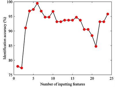
Fig. 17The optimization results of SVM parameters with GA

5.3. The result of fault diagnosis

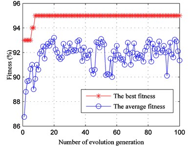
The sensitive feature set of training sample is fed into SVM. In order to obtain better generalization performance, GA is performed to optimize parameters of SVM. In the process of optimization, the number of termination generation is set as 100 and the initial population quantity is set as 20. The fitness diagram of GA is shown in Fig. 17. We can find that the best fitness of training sample is 95 %. The optimization result is that the kernel function parameter $g =$ 73.3481, and the penalty factor $c =$ 62.4312.

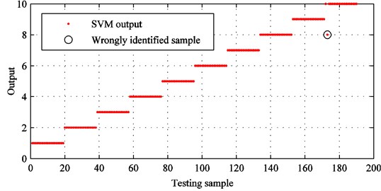
The trained SVM model is applied to identify rolling bearing fault conditions, and the identification results are shown in Fig. 18. It can be seen that the final identification accuracy is 99.4737 % and only one of the 190 samples is misclassified. Hence, it demonstrates that the proposed method is able to accurately identify rolling bearing fault conditions.

Fig. 18SVM identification results with improved CEEMDAN and sensitive feature set

5.4. Comparison and analysis

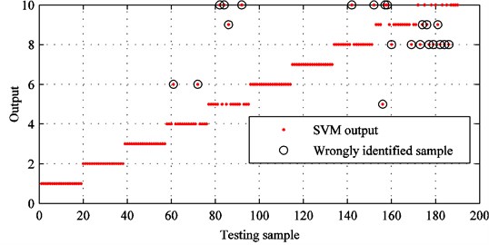
1) In order to highlight the advantages of improved CEEMDAN, conventional EMD and improved CEEMDAN are utilized to process vibration signals of rolling bearing, respectively. Original feature set is extracted from the first eight IMFs and taken as the input of SVM. GA is applied to optimize SVM parameters. The ultimate identification results of improved CEEMDAN and conventional EMD are presented in Fig. 19 and Fig. 20.

From Fig. 19, it can be seen that the identification accuracy of improved CEEMDAN is 95.7895 % and 8 samples are wrongly identified. In contrast, there are 22 samples are identified by error and the identification accuracy is 88.4211 % by employing conventional EMD. In detail, the accuracy of fault diagnosis decreases by 7.3684 %. Thus, it demonstrates that improved CEEMDAN is an effective tool for processing rolling bearing vibration signals.

2) To verify the effectiveness of distance evaluation technique, the identification results are compared by using the aforementioned two kinds of feature sets based on improved CEEMDAN.

From Fig. 18 and Fig. 19, we can find that the sensitive feature set increases the identification accuracy by 3.6842 %. The comparison indicates that distance evaluation technique can discard irrelevant features and enhance identification accuracy effectively. Thus, it is appropriate for fault diagnosis which needs to deal with large amounts of data.

Fig. 19SVM identification results with improved CEEMDAN and original feature set

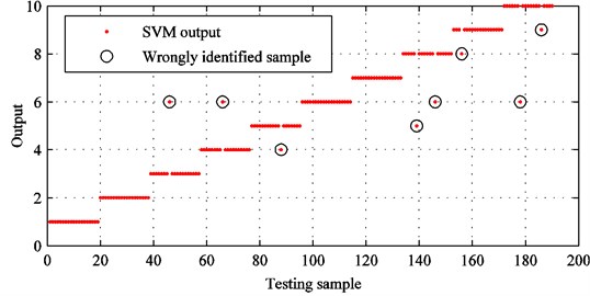
Fig. 20SVM identification results with conventional EMD and original feature set

6. Conclusions

1) Vibration signals of rolling bearing are decomposed by improved CEEMDAN and the first eight IMFs are selected for extracting fault features. Then the original feature set is obtained including energy values, singular values and envelope sample entropy values. It can reveal rolling bearing fault conditions entirely, and the underlying fault information can be excavated from different aspects.

2) Distance evaluation technique is implemented for selecting sensitive feature set, and irrelevant or redundant features can be discarded. By using sensitive feature set, the computational efficiency of classifier is enhanced and identification accuracy can be improved effectively.

3) The simulation experiment indicates that improved CEEMDAN is able to eliminate the mode mixing phenomenon and achieve negligible reconstruction error. In the meantime, the proposed method is utilized to identify different rolling bearing fault conditions. The experimental results demonstrate that improved CEEMDAN can increase the identification accuracy by 7.3684 % based on the original feature set. Moreover, the sensitive feature set can further enhance the identification accuracy by 3.6842 % based on improved CEEMDAN. Thus, it provides a new approach for rolling bearing fault diagnosis.

References

Straczkiewicz M., Czop P., Barszcz T. The use of a fuzzy logic approach for integration of vibration-based diagnostic features of rolling element bearings. Journal of Vibroengineering, Vol. 17, Issue 4, 2015, p. 1760-1768.

Search CrossRef
Siegel D., AI-Atat H., Shauche V., et al. Novel method for rolling element bearing health assessment – A tachometer-less synchronously averaged envelope feature extraction technique. Mechanical Systems and Signal Processing, Vol. 29, 2012, p. 362-376.

Publisher
Qu L. S., Zhang X. N., Shen Y. D. The Theory and Method of Mechanical Fault Diagnosis. Xi’an Jiaotong University Press, Xi’an, 2008, (in Chinese).

Search CrossRef
Wang Y., Xu G. H., Luo A. L., et al. An online tacholess order tracking technique based on generalized demodulation for rolling bearing fault detection. Journal of Sound and Vibration, Vol. 367, 2016, p. 233-249.

Publisher
Yu D. J. The Hilbert-Huang Transform Method of Mechanical Fault Diagnosis. Science Press, Beijing, 2007, (in Chinese).

Search CrossRef
Yang Y., Yu D. J., Chen J. S. Rolling bearing fault diagnosis method based on EMD and neural network. Journal of Vibration and Shock, Vol. 24, Issue 1, 2005, p. 85-88, (in Chinese).

Search CrossRef
Hassan A. R., Bhuiyan M. I. H. Automatic sleep scoring using statistical features in the EMD domain and ensemble methods. Biocybernetics and Biomedical Engineering, Vol. 36, Issue 1, 2016, p. 248-255.

Publisher
Lee Y. K., Tang S. C., Yeh J. R., et al. Detecting signal quality by ensemble empirical mode decomposition and Monte Carlo verification. Biomedical Signal Processing and Control, Vol. 20, 2015, p. 10-15.

Publisher
Aied H., Gonzalez A., Cantero D. Identification of sudden stiffness changes in the acceleration response of a bridge to moving loads using ensemble empirical mode decomposition. Mechanical Systems and Signal Processing, Vol. 66, Issue 67, 2016, p. 314-338.

Publisher
Imaouchen Y., Kedadouche M., Alkama R., et al. A frequency-weighted energy operator and complementary ensemble empirical mode decomposition for bearing fault detection. Mechanical Systems and Signal Processing, Vol. 82, 2017, p. 103-116.

Publisher
Zhao L. Y., Yu W., Yan R. Q. Gearbox fault diagnosis using complementary ensemble empirical mode decomposition and permutation entropy. Shock and Vibration, Vol. 2016, 2016, p. 1-8.

Publisher
Torres M. E., Colominas M. A., Schlotthauer G., et al. A complete ensemble empirical mode decomposition with adaptive noise. Proceedings of the 36th IEEE International Conference on Acoustics, Speech and Signal Processing, 2011, p. 4144-4147.

Publisher
Hassan A. R., Bhuiyan M. I. H. Computer-aided sleep staging using complete ensemble empirical mode decomposition with adaptive noise and bootstrap aggregating. Biomedical Signal Processing and Control, Vol. 24, 2016, p. 1-10.

Publisher
Afanasyev D. O., Fedorova E. A. The long-term trends on the electricity markets: comparison of empirical mode and wavelet decompositions. Energy Economics, Vol. 56, 2016, p. 432-442.

Publisher
Colominas M. A., Schlotthauer G., Torres M. E. Improved complete ensemble EMD: A suitable tool for biomedical signal processing. Biomedical Signal Processing and Control, Vol. 14, 2014, p. 19-29.

Publisher
Yayli M. O. On the axial vibration of carbon nanotubes with different boundary conditions. Micro and Nano Letters, Vol. 9, Issue 11, 2014, p. 807-811.

Publisher
Yayli M. O. Free vibration behavior of a gradient elastic beam with varying cross section. Shock and Vibration, Vol. 2014, 2014, p. 1-11.

Publisher
Tian Y., Ma J., Lu C., et al. Rolling bearing fault diagnosis under variable conditions using LMD-SVD and extreme learning machine. Mechanism and Machine Theory, Vol. 90, 2015, p. 175-186.

Publisher
Cong F. Y., Zhong W., Tong S. G., et al. Research of singular value decomposition based on slip matrix for rolling bearing fault diagnosis. Journal of Sound and Vibration, Vol. 344, 2015, p. 447-463.

Publisher
Carbajo E. S., Carbajo R. S., McGoldrick C., et al. ASDAH: An automated structural change detection algorithm based on the Hilbert-Huang transform. Mechanical Systems and Signal Processing, Vol. 47, Issues 1-2, 2014, p. 78-93.

Publisher
Qu J. X., Zhang Z. S., Wen J. P., et al. State recognition of the viscoelastic sandwich structure based on the adaptive redundant second generation wavelet packet transform, permutation entropy and the wavelet support vector machine. Smart Materials and Structures, Vol. 23, Issue 8, 2014, p. 085004.

Publisher
Zeng K., Yan J. Q., Wang Y. H., et al. Automatic detection of absence seizures with compressive sensing EEG. Neurocomputing, Vol. 171, 2016, p. 497-502.

Publisher
Li M. L., Liang L., Wang S. A. Sensitive feature extraction of machine faults based on sparse representation. Journal of Mechanical Engineering, Vol. 49, Issue 1, 2013, p. 73-80.

Publisher
Li N., Zhou R., Hu Q. H., et al. Mechanical fault diagnosis based on redundant second generation wavelet packet transform, neighborhood rough set and support vector machine. Mechanical Systems and Signal Processing, Vol. 28, 2012, p. 608-621.

Publisher
Qu J. X., Zhang Z. S., Gong T. A novel intelligent method for mechanical fault diagnosis based on dual-tree complex wavelet packet transform and multiple classifier fusion. Neurocomputing, Vol. 171, 2016, p. 837-853.

Publisher
Lei Y. G., He Z. J., Zi Y. Y. A new approach to intelligent fault diagnosis of rotating machinery. Expert Systems with Applications, Vol. 35, Issue 4, 2007, p. 1593-1600.

Publisher
Lei Y. G., He Z. J., Zi Y. Y., et al. New clustering algorithm-based fault diagnosis using compensation distance evaluation technique. Mechanical Systems and Signal Processing, Vol. 22, Issue 2, 2008, p. 419-435.

Publisher
Hu Q., He Z. J., Zhang Z. S., et al. Fault diagnosis of rotating machinery based on improved wavelet package transform and SVMs ensemble. Mechanical Systems and Signal Processing, Vol. 21, Issue 2, 2007, p. 688-705.

Publisher
Widodo A., Yang B. S. Support vector machine in machine condition monitoring and fault diagnosis. Mechanical Systems and Signal Processing, Vol. 21, Issue 6, 2007, p. 2560-2574.

Publisher

Cited by

Time–Frequency Decomposition Based Protection Scheme for Power Transformer— Simulation and Experimental Validation

Het Bhalja | Bhavesh R. Bhalja | Pramod Agarwal | Om P. Malik

(2024)

Multi-cavitation states identification of a sewage pump using CEEMDAN and BOA-SVM

Peijian Zhou | Weitao Zeng | Wenwu Zhang | Chengui Zhou | Zhifeng Yao

(2024)

Modified Complete Ensemble Empirical Mode Decomposition based HIF detection approach for microgrid system

Monalisa Biswal | Ch. Durga Prasad | Papia Ray | Nand Kishor

(2022)

Comparative study between objective and subjective methods for identifying the gravity of single and multiple gear defects in case of noisy signals

Zakarya Ouelaa | Ramdane Younes | Abderrazek Djebala | Nacer Hamzaoui | Nouredine Ouelaa

(2022)

Multifaceted irradiance prediction by exploiting hybrid decomposition-entropy-Spatiotemporal attention based Sequence2Sequence models

(2022)

An adaptive time–frequency approach based secured back-up distance protection scheme for system stress conditions

Fanidhar Dewangan | Monalisa Biswal

(2022)

Roller bearing fault diagnosis based on LMD and multi-scale symbolic dynamic information entropy

Minghong Han | Yaman Wu | Yumin Wang | Wei Liu

(2021)

A Fault Feature Extraction Method of Motor Bearing Using Improved LCD

Feng Ding | Xinrui Zhang | Wenfeng Wu | Yihua Wang

(2020)

Fault diagnosis of rolling bearings in non-stationary running conditions using improved CEEMDAN and multivariate denoising based on wavelet and principal component analyses

Lilia Chaabi | Ahcene Lemzadmi | Abderrazek Djebala | Mohamed Lamine Bouhalais | Nouredine Ouelaa

(2020)

Fault Feature Extraction and Diagnosis of Rolling Bearings Based on Wavelet Thresholding Denoising with CEEMDAN Energy Entropy and PSO-LSSVM

Wuge Chen | Junning Li | Qian Wang | Ka Han

(2020)

Advances in Asset Management and Condition Monitoring

Feng Ding | Xuejiao Chen | Jianhui Tian | Wenjuan Wang

(2020)

Comparative study between cyclostationary analysis, EMD, and CEEMDAN for the vibratory diagnosis of rotating machines in industrial environment

(2020)

Dynamic analysis of localized defects in rolling bearing systems

Mengmeng Song | Shungen Xiao | Lixia Huang | Wanxiang Li

(2017)

About this article

Received

12 July 2016

Accepted

14 October 2016

Published

15 February 2017

SUBJECTS

Fault diagnosis based on vibration signal analysis

DOI

https://doi.org/10.21595/jve.2016.17398

Keywords

rolling bearing

fault diagnosis

improved complete ensemble empirical mode decomposition with adaptive noise (CEEMDAN)

distance evaluation technique

Acknowledgements

This research is financially supported by the National Science Foundation of China (Grant No. 51275374) and the Fund Project of Science and Technology on Reliability and Environmental Engineering Key Laboratory.

This is an open access article distributed under the Creative Commons Attribution License, which permits unrestricted use, distribution, and reproduction in any medium, provided the original work is properly cited.

Previous article in issue Previous Next article in issue Next

Research article

2024 01 21

Rolling bearing fault diagnosis based on variational mode decomposition and weighted multidimensional feature entropy fusion

Na Lei, Feihu Huang, Chunhui Li

Research article

2023 08 01

Rolling bearing fault diagnosis method based on ELMD hybrid feature extraction and wavelet neural network

Hengxin Yue, Xihui Chen, Xinhui Shi, Wei Lou

Review article

2021 11 26

Fault diagnosis and health management of bearings in rotating equipment based on vibration analysis – a review

Adnan Althubaiti, Faris Elasha, Joao Amaral Teixeira

Research article

2021 02 04

Fault diagnosis of rolling bearings based on improved enhanced envelope spectrum

Baoyu Huang, Yongxiang Zhang, Danchen Zhu

F. Ding, X. Li, and J. Qu, “Fault diagnosis of rolling bearing based on improved CEEMDAN and distance evaluation technique,” Journal of Vibroengineering, Vol. 19, No. 1, pp. 260–275, Feb. 2017, https://doi.org/10.21595/jve.2016.17398

Copy Extrica

Copied to clipboard!

TY  - JOUR
DO  - 10.21595/jve.2016.17398
UR  - https://doi.org/10.21595/jve.2016.17398
TI  - Fault diagnosis of rolling bearing based on improved CEEMDAN and distance evaluation technique
T2  - Journal of Vibroengineering
AU  - Ding, Feng
AU  - Li, Xiang
AU  - Qu, Jinxiu
PY  - 2017
DA  - 2017/02/15
PB  - JVE International Ltd.
SP  - 260-275
IS  - 1
VL  - 19
SN  - 1392-8716
ER  - 

Copy Ris

Copied to clipboard!

@article{Ding_2017,
	doi = {10.21595/jve.2016.17398},
	url = {https://doi.org/10.21595/jve.2016.17398},
	year = 2017,
	month = {feb},
	publisher = {{JVE} International Ltd.},
	volume = {19},
	number = {1},
	pages = {260--275},
	author = {Feng Ding and Xiang Li and Jinxiu Qu},
	title = {Fault diagnosis of rolling bearing based on improved {CEEMDAN} and distance evaluation technique},
	journal = {Journal of Vibroengineering}
}

Copy Bibtex

Copied to clipboard!

[1]F. Ding, X. Li, and J. Qu, “Fault diagnosis of rolling bearing based on improved CEEMDAN and distance evaluation technique,” Journal of Vibroengineering, vol. 19, no. 1, pp. 260–275, Feb. 2017, doi: 10.21595/jve.2016.17398.

Copy IEEE

Copied to clipboard!

Ding, Feng, Xiang Li, and Jinxiu Qu. “Fault Diagnosis of Rolling Bearing Based on Improved CEEMDAN and Distance Evaluation Technique.” Journal of Vibroengineering 19, no. 1 (February 15, 2017): 260–75. https://doi.org/10.21595/jve.2016.17398.

Copy Chicago

Copied to clipboard!

Fault diagnosis of rolling bearing based on improved CEEMDAN and distance evaluation technique

Abstract

1. Introduction

2. Improved CEEMDAN

2.1. Algorithm of improved CEEMDAN

2.2. Evaluation and comparison of EEMD, CEEMDAN and improved CEEMDAN

3. Feature extraction and selection

3.1. Feature extraction based on improved CEEMDAN

3.1.1. Energy feature

3.1.2. Singular value feature

3.1.3. Envelope sample entropy feature

3.2. Sensitive feature selection based on distance evaluation technique

4. The procedure of rolling bearing fault diagnosis

5. Experiment verification

5.1. Signal processing and feature extraction

5.2. Sensitive feature selection

5.3. The result of fault diagnosis

5.4. Comparison and analysis

6. Conclusions

References

Cited by

About this article

Related Articles