Structural multi-damage identification based on strain energy and micro-search artificial fish swarm algorithm

Guo, Huiyong

doi:10.21595/jve.2017.17503

Journal of Vibroengineering

Browse Journal

Submit article

Published: 15 August 2017

Check for updates

Structural multi-damage identification based on strain energy and micro-search artificial fish swarm algorithm

Huiyong Guo¹

¹School of Civil Engineering, Chongqing University, Chongqing 400045, P. R. China

¹Key Laboratory of New Technology for Construction of Cities in Mountain Area, Ministry of Education, Chongqing 400045, China

Cite the article Download PDF

Downloads 1462

WoS Core Citations 4

CrossRef Citations 2

Abstract

A two-stage damage detection method based on strain energy and micro-search artificial fish swarm algorithm (MSAFSA) is presented for solving structural multi-damage problem. First, structural modal strain energy and energy dissipation process are analyzed and an improved modal strain energy dissipation ration index (IMSEDRI) is proposed to preliminarily detect suspected damage elements. Then, artificial fish swarm algorithm (AFSA) is used to identify damage extent of suspected damage elements. In general, the search efficiency of a basic AFSA isn’t very efficient for the search procedure. So, a micro-search artificial fish swarm algorithm is presented in this paper. The simulation results demonstrate that the damage detection method can estimate the damage locations and extent with good accuracy, and the calculated results of the proposed MSAFSA are obviously superior to those of both the basic AFSA and the AFSA with visual-step change strategy.

1. Introduction

Structural damage identification has received increasing attention in the research community in recently two decades. It has become an important and rapidly growing research area, involving civil engineering, mechanical engineering, and aeronautical engineering with the goal of assessing the health condition and the dynamic characteristics of a structure. Most of the damage identification research focuses on dynamic characteristics which can be acquired from results of dynamic testing. The main dynamic characteristics include natural frequencies, mode shapes, modal strain energy etc. Natural frequency has already been used to detect structural damage. Cawley et al. [1] described a numerical method for detecting structural damage location through the measurements of natural frequencies. Salawu [2] identified structural damage through frequency changes. Chaudhari et al. [3] and Chinchalkar et al. [4] proposed a numerical method for determining the location of a crack in a beam of varying depth when the lowest three natural frequencies of the cracked beam are considered. Zhang et al. [5] utilized the natural frequencies to detect the delamination damage. However, the natural frequencies are not sensitive to local damage and the number of measured frequencies is few [2]. Mode shape or modal strain energy can also be utilized to detect structural damage [6-8]. Allemang et al. [9] presented a modal assurance criterion method, which detect damage through comparing mode shapes. Pindey and Biswas [10] identified structural damage by solving the linear damage equations of complete mode shapes. In general, modal strain energy method is more efficient than some mode shape methods for damage identification [11-13]. Shi et al. [14] proposed a modal strain energy change index to assess the damage state of a structure. Sazonov et al. [15] studied vibration-based methods of non-destructive damage detection by utilizing curvature or strain energy mode shapes. Liu et al. [16] presented a modal strain energy dissipation ratio index (MSEDRI), which can approximately detect structural damage sites. It is necessary for the MSEDRI to calculate the modal strain energy change value in each element. However, the MSEDRI didn’t consider the modal strain energy change tendency to damage. Therefore, an improved modal strain energy dissipation ratio index will be proposed.

Artificial fish swarm algorithm is a new population-based swarm intelligent evolutionary computation technique proposed by Li et al. [17] that was inspired by the natural schooling behavior of fish. AFSA presents a strong ability to avoid local minimums in order to achieve global optimization. It has been proofed in function optimization, parameter estimation, combinatorial optimization, least squares support vector machine and geotechnical engineering problems [18, 19]. AFSA imitates three typical behaviors, defined to include “searching for food”, “swarming in response to a threat”, and “following to increase the chance of achieving a successful result”. Three major parameters involved in AFSA include visual distance (visual), maximum step length (step), and a crowd factor [17]. Here, The AFSA is proposed to detect structural damage locations and extent. In general, it is difficult for the basic AFSA to identify the multi-damage problem of complex structure. Therefore, a micro-search artificial fish swarm algorithm (MSAFSA) is presented to improve identification capability.

In this study, a two-stage damage detection method based on micro-search artificial fish swarm algorithm and IMSEDRI is proposed. First, an improved modal strain energy dissipation ration index is proposed to identify suspected damage elements. Then, after the suspected damage elements are preliminarily determined, the micro-search artificial fish swarm algorithm is presented to find the damage severity of the suspected damage elements. There are seven sections in this paper. Section 2 introduces strain energy and energy dissipation process, and presents the improved modal strain energy dissipation ration index. Section 3 briefly describes an artificial fish swarm algorithm. Section 4 proposes some improved strategies and presents the micro-search artificial fish swarm algorithm. Section 5 introduces the two-stage method based on artificial fish swarm algorithm and IMSEDRI. Section 6 gives numerical examples. Finally, Section 7 presents the conclusions.

2. Improved modal strain energy dissipation ration index

Modal strain energy can be used to detect structural damage. The modal strain energy of the $j$ th element and the $i$ th mode before and after the occurrence of damage is expressed as:

1a

M S E_{i j}^{u} = \frac{1}{2} Φ_{i}^{T} K_{j} Φ_{i},

1b

M S E_{i j}^{d} = \frac{1}{2} Φ_{i}^{d T} K_{j} Φ_{i}^{d} .

In which $M S E_{i j}^{u}$ is the undamaged modal strain energy (MSE); $Φ_{i}$ is the $i$ th undamaged mode shape; $M S E_{i j}^{d}$ is the damaged MSE; $Φ_{i}^{d}$ is the $i$ th damaged mode shape; $K_{j}$ is the stiffness matrix of the $j$ th element. When the first $m$ mode shapes are considered, the undamaged and damaged modal strain energy of the $j$ th element can be given by:

2a

M S E_{j}^{u} = \frac{1}{2} \sum_{i = 1}^{m} Φ_{i}^{T} K_{j} Φ_{i},

2b

M S E_{j}^{d} = \frac{1}{2} \sum_{i = 1}^{m} Φ_{i}^{d T} K_{j} Φ_{i}^{d} .

If:

3

u_{j} = M S E_{j}^{u}, d_{j} = M S E_{j}^{d} .

Thus, the modal strain energy change of the $j$ th element is simply expressed as:

4

M S E C_{j} = d_{j} - u_{j} .

Damage will cause the change of MSE. In general, damage can also be described as energy dissipation process [20]. The same damage will cause the same energy change. Therefore, the modal strain energy change caused by damage should be equal to the energy dissipation caused by the same damage.

Structural damage is also the energy dissipation process. The strain energy dissipation ratio at time $t$ is described as follows [20]:

5

φ (t) = \frac{- \dot{c} (t)}{{[1 - c (t)]}^{2}} \int_{V} (σ^{T} ε) d V .

In which $t$ is time; $σ$ is the stress vector; $ε$ is the strain vector; $V$ is the volume; $c$ is damage coefficient. Structural damage can be described as the energy dissipation process of undamaged system. Thus, the strain energy dissipation ratio of the $j$ th element can be expressed as:

6

φ_{j} (t) = \frac{- {\dot{c}}_{j} (t)}{{[1 - c_{j} (t)]}^{2}} u_{j} .

When $t =$ 0, no damage occurs; when $t = t^{d}$ , damage occurs. It can be hypothesized that there is a linear relationship between $c_{j} (t)$ and $t$ . Thus, the derivative ${\dot{c}}_{j} (t)$ is a constant. If a damage $c_{j}$ occurs in the $j$ th element, the energy dissipation of the $j$ th element can be given by:

7

\int_{0}^{t^{d}} φ_{j} (t) d t = u_{j} \int_{0}^{t^{d}} \frac{- {\dot{c}}_{j} (t)}{{[1 - c_{j} (t)]}^{2}} d t = u_{j} \frac{- c_{j}}{1 - c_{j}} .

The same damage will cause the same energy change. Therefore, the modal strain energy change should be equal to the energy dissipation caused by the same damage. Considering Eqs. (4) and (7), the following equation can be obtained:

8

|d_{j} - u_{j}| = |u_{j} \frac{- c_{j}}{1 - c_{j}}| .

Thus, the modal strain energy dissipation ration index [16] of the $j$ th element is obtained as follow:

9

M S E D R I_{j} = \frac{|M S E_{j}^{d} - M S E_{j}^{u}|}{|M S E_{j}^{d} - M S E_{j}^{u}| + M S E_{j}^{u}} .

In general, damage will cause the stiffness degradation, and it will also cause the increase of modal strain energy [21]. Therefore, an improved modal strain energy dissipation ration index (IMSEDRI) is given by:

10

I M S E D R I_{j} = m a x [0, \frac{M S E_{j}^{d} - M S E_{j}^{u}}{|M S E_{j}^{d} - M S E_{j}^{u}| + M S E_{j}^{u}}] .

Thus, incorrect index value can be directly excluded. From Eq. (10), we can find the suspected damage elements. After the suspected damage elements are preliminarily identified, the damage extent can be determined by using an artificial fish swarm algorithm.

3. Artificial fish swarm algorithm

Artificial fish swarm algorithm (AFSA) is a new population-based optimization technique inspired by the natural feeding behavior of fish, which was first proposed by Li et al. [17]. In general, a fish is represented by its $N$ -dimensional position $X_{i} = (x_{1}, x_{2}, \dots, x_{N},)$ , and $Y (X_{i})$ is the fitness or objective function at position $X_{i}$ . The relationship between two fish is denoted by their Euclidean distance $‖X_{j} - X_{i}‖$ . Visual and Step stand for the perception range and the moving step of the artificial fish, respectively. The basic fish-swarm behaviors include foraging behavior, swarming behavior, following behavior and random behavior.

3.1. Foraging behavior

Foraging is a basic biological behavior adopted by fish looking for food. Let $X_{i}$ be the current state of an artificial fish, and select a state $X_{j}$ randomly in its Visual range. For the minimization problem, if $Y_{j} < Y_{i}$ , the artificial fish moves a step in the direction of $(X_{j} - X_{i})$ . Otherwise, select a state $X_{j}$ randomly again and judge whether it satisfies the forward condition. If it cannot be satisfied after try-number times, the random behavior is performed. The foraging behavior is expressed mathematically as:

11

X_{n e x t} = \{\begin{array}{l} X_{i} + \frac{X_{j} - X_{i}}{‖X_{j} - X_{i}‖} \times s t e p \times r a n d, & (Y_{j} < Y_{i}), \\ random behavior, & otherwise, \end{array}

where $X_{n e x t}$ is the next state of the artificial fish, $r a n d$ is uniformly distributed random number in the interval [0, 1].

3.2. Swarming behavior

In the fish swarm, each artificial fish should explore the central position $X_{c}$ of $n_{f}$ artificial fish in its neighborhood ( $d_{i j} < V i s u a l$ ). If $Y_{c} \cdot n_{f} < δ \cdot Y_{i}$ (For the minimization problem), the artificial fish $X_{i}$ will go forward a step to the $X_{c}$ . It is expressed mathematically as:

12

X_{n e x t} = \{\begin{array}{l} X_{i} + \frac{X_{c} - X_{i}}{‖X_{c} - X_{i}‖} \times s t e p \times r a n d, & (Y_{c} \cdot n_{f} < δ \cdot Y_{i}), \\ foraging behavior, & otherwise . \end{array}

In which $δ$ is the food concentration or crowd factor.

3.3. Following behavior

Let $X_{i}$ be the current state of an artificial fish, and $X_{m i n}$ (for minimization problem) is the best companion in the current neighborhood of $X_{i}$ If $Y_{m i n} \cdot n_{f} < δ \cdot Y_{i}$ (For the minimization problem), the artificial fish $X_{i}$ will go forward a step to the $X_{m i n}$ . The following behavior is given by:

13

X_{n e x t} = \{\begin{array}{l} X_{i} + \frac{X_{m i n} - X_{i}}{‖X_{m i n} - X_{i}‖} \times s t e p \times r a n d, & (Y_{m i n} \cdot n_{f} < δ \cdot Y_{i}), \\ foraging behavior, & otherwise . \end{array}

3.4. Random behavior

The artificial fish select a position randomly in its Visual range, and then it moves towards the position. The random behavior can be written as:

14

X_{n e x t} = X_{i} + V i s u a l \times s t e p \times r a n d .

In addition, artificial fish swarm algorithm will provide a bulletin to record the optimal state in the fish swarm. Each artificial fish compares its own state with the bulletin after making a step. If its state is better, the bulletin will be updated.

4. Micro-search artificial fish swarm algorithm

In general, the search efficiency of the basic AFSA isn’t very high. Therefore, it is necessary to modify the basic AFSA. Here, some improved strategies are proposed and micro-search artificial fish swarm algorithm is presented.

4.1. Visual-step change strategy

Visual and Step have an important effect on AFSA [18, 19]. Therefore, an artificial fish swarm algorithm with visual-step change strategy is proposed. The method mainly presented novel Visual equation and Step equation.

The novel Visual equation and Step equation are expressed mathematically as:

15

V i s u a l = V i s u a l_{0} - p \times V i s u a l_{0} \times \frac{t p}{m},

16

S t e p = S t e p_{0} - q \times S t e p_{0} \times \frac{t p}{m},

where, $V i s u a l_{0}$ is initial value of visual distance; $p$ is change parameter of visual distance; $t p$ is the current iteration number; $m$ is the total iteration number; $S t e p_{0}$ is initial value of step length; $q$ is change parameter of step length. Thus, the visual and step will dynamically change with the iteration number. In general, the AFSA with visual-step change strategy can improve the search efficiency.

4.2. Micro-search strategy

The best location of fish in a swarm is picked out and this location is called as elitist state. Then, the elitist state will be further optimized by using the micro-search strategy. Here, we assumed the identification precision of damage is 1 %. Thus, the micro-search distance is equal to 0.01. The fish will move ±0.01 micro-search step in turn. The method is shown in Fig. 1.

Fig. 1Micro-search of the elitist state

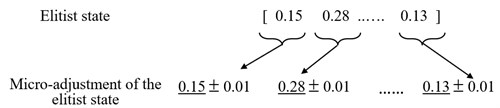
If the elitist state is understood as a location in $n$ -dimensional space, the elitist state should contain $n$ components. We will adjust all the $n$ components by ±0.01 steps in turn. Thus, we will search all the potential change in the $n$ components. If the generated elitist state is better than the original elitist state, the original elitist state will be replaced by the generated elitist state. Finally, the best state is recorded in bulletin. If the elitist state isn’t change in the next generation, the micro-search should be omitted to avoid the redundant calculation. Therefore, the micro-search strategy can easily find the best solution and improve the search efficiency.

4.3. Two termination criteria.

Two termination criteria are expressed as follows: Eq. (1) If the optimal state in the bulletin does not change in continuous $t_{1}$ iterations, the iteration process will be terminated. The termination number $t_{1}$ can avoid redundant iteration calculation. Eq. (2) If the calculation value of the optimal state is 0 or a very small number, which means that the optimal solution has been obtained, the iteration process will be terminated. Either of the two termination criteria is met, the iteration calculation will be ended.

The artificial fish swarm algorithm with the three improved strategies is called as micro-search artificial fish swarm algorithm (MSAFSA). The flowchart of the MSAFSA is shown in Fig. 2 and is summarized as follows:

Fig. 2Flowchart of MSAFSA

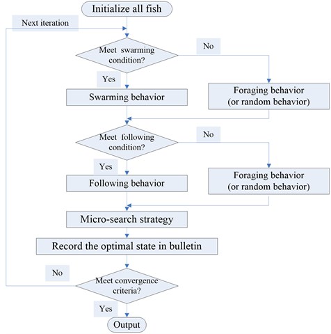
Step 1: Create all fish, and calculate the objective function of the location state of the fish.

Step 2: Perform swarming behavior if the swarming condition is met. Otherwise, perform foraging behavior or random behavior.

Step 3: Perform following behavior if the following condition is met. Otherwise, perform foraging behavior or random behavior.

Step 4: Pick out the best fish of a swarm, and update the elitist state by using micro-search strategy. If the elitist state isn’t adjusted in the next generation, the micro-search process will be ignored.

Step 5: Record the optimal state in the fish swarm in bulletin.

Step 6: Repeat Step 2-Step 5 until either of the two termination criteria is met.

5. Damage identification based on artificial fish swarm algorithm

It is difficult for artificial fish swarm algorithm to detect multiple damage of a complex structure. Here, we propose a two-stage damage identification method. First, the improved modal strain energy dissipation ration index is used to preliminarily identify the suspected damage elements. Then, the artificial fish swarm algorithm is utilized to find the damage extent of the suspected damage elements. A structure consists of $N E$ elements. If we find $N D$ suspected damage elements in the $N E$ elements by using the IMSEDRI, we just need identify the damage extent of the $N D$ suspected elements by using the AFSA $(N D < N E)$ . Thus, when the identification precision of damage extent is 1 %, the search space consists of 101 $N D$ different kinds of damage extent and we just need to find the optimal solution from 101 $N D$ different kinds of damage extent. If we directly utilize the AFSA to search true damage extent of the $N E$ elements, we need to find the optimal solution from 101 $N E$ different kinds of damage extent. In general, $101 N D < < 101 N E$ . Therefore, the proposed two-stage method is of better convergence and higher search efficiency.

The objective function of the artificial fish swarm algorithm is given by:

17

J = 2 - \frac{{|{\{Δ f\}}^{T} \cdot \{δ f (\{δ D\})\}|}^{2}}{({\{Δ f\}}^{T} \cdot \{Δ f\}) \cdot (δ f {(\{δ D\})}^{T} \cdot δ f (\{δ D\}))} - \frac{{|{\{Δ Φ\}}^{T} \cdot \{δ Φ (\{δ D\})\}|}^{2}}{({\{Δ Φ\}}^{T} \cdot \{Δ Φ\}) \cdot (δ Φ {(\{δ D\})}^{T} \cdot δ Φ (\{δ D\}))},

where, $\{∆ f\}$ is the change vector of measured frequency; $\{δ D\}$ is the theoretical damage degree of suspected damage elements; $\{δ f (\{δ D\})\}$ is the change vector of theoretical frequency for damage on $\{δ D\}$ ; $\{∆ Ф\}$ is the change vector of measured mode shape; $\{δ Ф (\{δ D\})\}$ is the change vector of theoretical mode shape for damage on $\{δ D\}$ .

Here, the suspected damage vector $\{δ D\}$ can be obtained by using the improved modal strain energy dissipation ration index. The best objective function value should be 0 or a small value. Therefore, this is a minimization problem.

6. Numerical examples

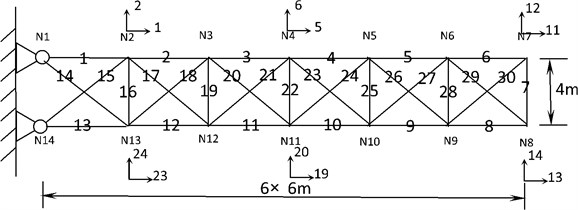
In order to investigate the effectiveness of the two-stage method, a two-dimensional truss structure has been used. The size of the truss structure is depicted in Fig. 3. The material property of the structure is: $ρ =$ 2800 kg/m³, $E =$ 72 GPa, and $A =$ 0.001 m². The truss model consists of 30 bar elements, 14 nodes, and 24 degrees of freedom. Damage is simulated by a reduction in the stiffness of individual bars in the structure. Damage cases are shown in Table 1. The parameters of MSAFSA are: $V i s u a l_{0} =$ 0.4; change parameter of visual distance $p =$ 0.8; $S t e p_{0} =$ 0.4; change parameter of step length $q =$ 0.9; crowd factor $δ =$ 0.2; identification precision is 0.01; micro-search distance is 0.01; termination parameter $t_{1}$ is 20; total number of fish is 100; maximum iteration number is 100.

Fig. 3Two-dimensional truss structure

It is important to determine suspected damage elements in the damage identification process. If the number of suspected damage elements can be effectively reduced, it will be easy to find the true damage elements and extent by using artificial fish swarm algorithm. Therefore, the IMSEDRI is used to identify suspected damage elements. For a given set of suspected damage elements, the true damage extent is calculated by using the MSAFSA. In order to compare and contrast different artificial fish swarm algorithms, the basic AFSA and the AFSA with visual-step change strategy are also utilized to identify structural damage. The first ten natural frequencies and three mode shapes are applied to calculate the objective function of the algorithms.

Table 1Damage cases for two-dimensional truss

Case 1		Case 2
Element No. (1)	Damage (2)	Element No. (3)	Damage (4)
5	25 %	7	15 %
8	15 %	9	20 %
25	15 %	28	20 %

6.1. Case 1

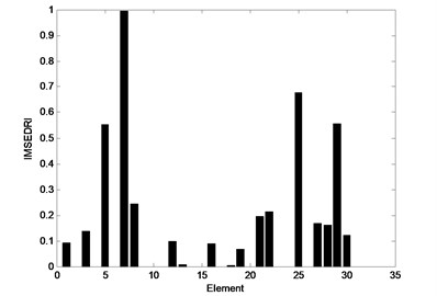
In general, damage can be considered as the stiffness reduction. In this case, elements 5, 8 and 25 have 25 %, 15 % and 15 % stiffness reduction, respectively. The calculation procedure of the method is depicted as follows: First, the improved modal strain energy dissipation ration index is utilized to find suspected damage elements. Then, the highest five elements are selected as suspected damage elements. Finally, the AFSA is used to identify the damage extent of the suspected elements. The localization identification results of the IMSEDRI are shown in Fig. 4. An element with relatively higher IMSEDRI value means that it is more probable to be the true damage element. In general, with the increase of suspected damage elements, the calculation cost will rapidly increase. In this case, five elements meet identification requirement. Therefore, the highest five elements are selected as suspected damage elements. Thus, the elements 5, 8, 25, 26 and 28 are picked out.

Fig. 4Damage identification results of the IMSEDRI for Case 1

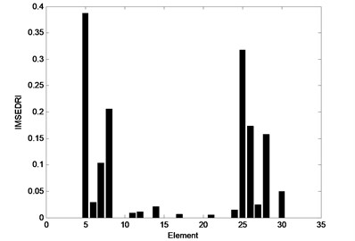
Table 2Quantitative results of 10 run using the basic AFSA for Case 1

No.	Elements and damage					Iteration number
No.	5	8	25	26	28	Iteration number
1	0.4300	0.2800	0.1500	0.0600	0.1500	29
2	0.5300	0.3100	0.1300	0.1700	0.0400	22
3	0.6000	0.3400	0	0	0.1600	68
4	0.2200	0.1300	0.1400	0	0	83
5	0.5000	0.0900	0.1500	0.1100	0.1500	22
6	0.6000	0.0600	0.1300	0.1900	0.1600	49
7	0.6000	0.3500	0.1600	0.0700	0.0400	22
8	0.4800	0.5400	0.0300	0.1700	0.1500	22
9	0.1500	0.1800	0.1300	0.0300	0.1100	23
10	0.6000	0.2700	0.0700	0.0100	0.1800	87
Average	0.471	0.255	0.109	0.081	0.114	42.7

Then, the basic AFSA, the AFSA with visual-step change strategy and the MSAFSA, are used to calculate the damage extent of the suspected elements. These algorithms only need to detect the damage extent of the five suspected elements 5, 8, 25, 26 and 28. The damage quantification results of 10 runs are shown in Tables 2-4. From Table 2, we can see that it is difficult for the basic AFSA to identify the true damage locations and extent. From Table 3, we can observe that the identification results of the AFSA with visual-step change strategy are close to the true damage extent, but the average iteration number is relatively higher. From Table 4, we can observe that the MSAFSA can find the true damage extent, and improve the convergence speed. Therefore, the MSAFSA is obviously superior to both the basic AFSA and the AFSA with visual-step change strategy.

Table 3Quantitative results of 10 run using the AFSA with visual-step change strategy for Case 1

No.	Elements and damage					Iteration number
No.	5	8	25	26	28	Iteration number
1	0.2000	0.0800	0.0100	0.0100	0.0100	57
2	0.1100	0.0500	0	0	0	44
3	0.2500	0.1500	0.1500	0	0	39
4	0.6000	0.3600	0.1300	0	0	30
5	0.3200	0.1900	0.1900	0	0.0100	68
6	0.2500	0.1500	0.1500	0	0	56
7	0.3100	0.1900	0.2000	0	0	74
8	0.0900	0.0500	0.0600	0	0.0100	78
9	0.1400	0.0800	0.0900	0	0	43
10	0.2500	0.1500	0.1500	0	0	71
Average	0.252	0.145	0.113	0.001	0.003	56

Table 4Quantitative results of 10 run using the MSAFSA for Case 1

No.	Elements and damage					Iteration number
No.	5	8	25	26	28	Iteration number
1	0.2500	0.1500	0.1500	0	0	55
2	0.2600	0.1500	0.1200	0	0.0100	31
3	0.2500	0.1500	0.1500	0	0	31
4	0.2500	0.1500	0.1500	0	0	19
5	0.2500	0.1500	0.1500	0	0	26
6	0.1700	0.1000	0.1000	0	0	31
7	0.2500	0.1500	0.1500	0	0	23
8	0.2500	0.1500	0.1500	0	0	25
9	0.2500	0.1500	0.1500	0	0	9
10	0.2500	0.1500	0.1500	0	0	26
Average	0.243	0.145	0.142	0	0.001	27.6

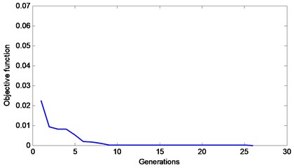
The representative objective function curves of the basic AFSA, AFSA with visual-step change strategy and MSAFSA, are depicted in Figs. 5-7, respectively. From Fig. 5, we can see that the objective function curve of the basic AFSA gradually tends to zero with the increasing number of generations. From Fig. 6, we can observe that the objective function curve of the AFSA with visual-step change strategy can quickly tends to zero, which show the effect of the dynamic visual and step. From Fig. 7, we can see that the objective function curve of the MSAFSA is quicker to tend to zero. The MSAFSA has the fastest convergence speed in the three algorithms. So, the MSAFSA is more effective than both the basic AFSA and the AFSA with visual-step change strategy.

In general, measurement error will affect the credibility of experimental data. Here, the frequencies with 0.15 % error and the mode shapes with 3 % error are considered. The IMSEDRI is used to identify suspected damage elements. The identification results of IMSEDRI with measurement error are depicted in Fig. 8. Here, we still select the highest five elements as suspected damage elements. So, the elements 5, 7, 8, 25 and 29 are picked out. The measurement error will also affect the identification results of the AFSAs.

Fig. 5An objective function curve of the basic AFSA for Case 1

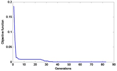
Fig. 6An objective function curve of the AFSA with visual-step change strategy for Case 1

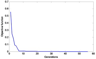
Fig. 7An objective function curve of the MSAFSA for Case 1

The basic AFSA, the AFSA with visual-step change strategy and the MSAFSA are used to assess the damage severity of the suspected damage elements. They only need to assess the damage severity of the suspected elements 5, 7, 8, 25, and 29. The calculation results are shown in Tables 5-7. From Table 5, we can see that the basic AFSA still cannot identify the true damage locations and extent. From Table 6, we can observe that the AFSA with visual-step change strategy can approximately find the true damage elements, but the iteration number is higher.

From Table 7, we can see that the MSAFSA can approximately find the true damage elements and improve the convergence speed. Therefore, the proposed MSAFSA is best one in the three algorithms.

Table 5Quantitative results of 10 run with measurement error using the basic AFSA for Case 1

No.	Elements and damage					Iteration number
No.	5	7	8	25	29	Iteration number
1	0.2700	0.0300	0.0200	0.1900	0.0100	22
2	0.2300	0.0600	0.1100	0.2100	0	61
3	0.2100	0.4100	0.1100	0.1900	0	65
4	0.2400	0	0.1000	0.1500	0	48
5	0.2200	0.5100	0.0900	0.1800	0	88
6	0.2200	0.2100	0.0800	0.1300	0.1000	96
7	0.2400	0.0200	0.1000	0.2000	0	56
8	0.2200	0.0400	0.1700	0.0300	0.0200	22
9	0.2400	0.2600	0.0900	0.1600	0.0300	76
10	0.2100	0.1900	0.1000	0.1900	0.1300	22
Average	0.23	0.173	0.097	0.163	0.029	55.6

Table 6Quantitative results of 10 run with measurement error using the AFSA with visual-step change strategy for Case 1

NO.	Elements and damage					Iteration number
NO.	5	7	8	25	29	Iteration number
1	0.2500	0	0.0900	0	0	43
2	0.2400	0	0.1000	0.1500	0	39
3	0.2400	0	0.1000	0.1500	0	48
4	0.2400	0.0900	0.1000	0.1500	0	50
5	0.2400	0	0.1000	0.1500	0	32
6	0.2400	0	0.1000	0.1500	0	32
7	0.2400	0.0100	0.1000	0.0100	0.0100	37
8	0.2400	0	0.1000	0.1500	0	32
9	0.2400	0.0900	0.1000	0.1500	0	66
10	0.2400	0	0.1000	0.1500	0	42
Average	0.241	0.019	0.099	0.121	0.001	42.1

Table 7Quantitative results of 10 run with measurement error using the MSAFSA for Case 1

No.	Elements and damage					Iteration number
No.	5	7	8	25	29	Iteration number
1	0.2400	0	0.1000	0.1600	0	8
2	0.2400	0.0100	0.1000	0.1500	0	9
3	0.2400	0	0.1000	0.1500	0	10
4	0.2400	0.0100	0.1000	0.1500	0	27
5	0.2400	0.0700	0.1000	0.1500	0	13
6	0.2400	0	0.1000	0.1500	0	30
7	0.2400	0.1400	0.1000	0.0600	0	52
8	0.2400	0	0.1000	0.1600	0	12
9	0.2400	0	0.1000	0.1500	0	16
10	0.2400	0.0700	0.1000	0.1500	0	14
Average	0.238	0.03	0.1	0.143	0	19.1

Fig. 8Damage identification results of the IMSEDRI with measurement error for Case 1

6.2. Case 2

In this case, elements 7, 9 and 28 have 15 %, 20 % and 20 % stiffness reduction, respectively. The IMSEDRI is used to detect suspected damage elements. The calculation results are depicted in Fig. 9. An element with relatively higher IMSEDRI value means that it is more probable to be the true damage element. Here, we still select the highest five elements as suspected damage elements. Thus, the elements 7, 8, 9, 27 and 28 are picked out. Then, the basic AFSA, the AFSA with visual-step change strategy and the MSAFSA are used to assess the damage severity of the suspected damage elements. They only need to assess the damage severity of the suspected elements 7, 8, 9, 27 and 28. The calculation results are shown in Tables 8-10. From Table 8, we can see that the basic AFSA can approximately detect the damage extent of suspected damage elements, but the average convergence speed isn’t very quick.

From Table 9, we can observe that the AFSA with visual-step change strategy can also approximately identify the damage extent, but the average convergence speed isn’t very quick yet. From Table 10, we can observe that the MSAFSA can find the true damage extent, and improve the convergence speed. So, it is obvious that the MSAFSA is better than both the basic AFSA and the AFSA with visual-step change strategy.

Fig. 9Damage identification results of the IMSEDRI for Case 2

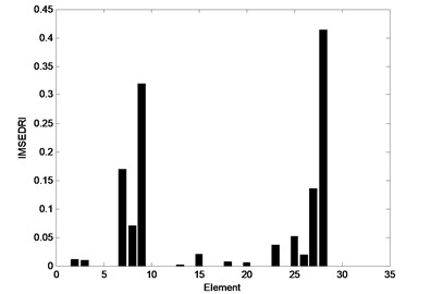
Table 8Quantitative results of 10 run using the basic AFSA for Case 2

No.	Elements and damage					Iteration number
No.	7	8	9	27	28	Iteration number
1	0	0.0100	0.2000	0	0.2000	49
2	0	0	0.2000	0	0.1900	37
3	0.5200	0.0200	0.1900	0	0.1700	40
4	0.1500	0	0.2000	0	0.2000	41
5	0.3400	0	0.2000	0	0.1800	45
6	0.1500	0	0.2000	0	0.2000	40
7	0	0	0.2000	0	0.1900	54
8	0.4300	0.0200	0.2200	0	0.0100	41
9	0.3500	0	0.2000	0	0.1700	62
10	0.1500	0	0.2000	0	0.2000	38
Average	0.209	0.005	0.201	0	0.171	44.7

Table 9Quantitative results of 10 run using the AFSA with visual-step change strategy for Case 2

No.	Elements and damage					Iteration number
No.	7	8	9	27	28	Iteration number
1	0.1500	0	0.2000	0	0.2000	38
2	0.3800	0	0.2000	0	0	36
3	0.3100	0	0.2000	0	0.1900	47
4	0.1500	0	0.2000	0	0.2000	30
5	0.3100	0	0.2000	0	0.1900	33
6	0	0	0.2000	0	0.1900	31
7	0.1500	0	0.2000	0	0.2000	45
8	0.1500	0	0.2000	0	0.2000	39
9	0.3100	0	0.2000	0	0.1900	46
10	0.1500	0	0.2000	0	0.2000	49
Average	0.206	0	0.2	0	0.176	39.4

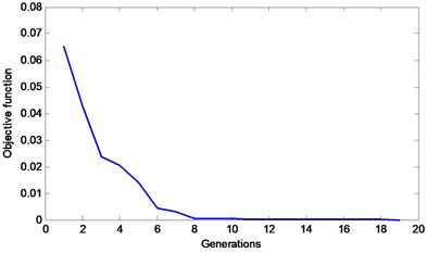
The representative objective function curves of the basic AFSA, AFSA with visual-step change strategy and MSAFSA, are depicted in Figs. 10-12, respectively. From Fig. 10, we can see that the objective function curve of the basic AFSA gradually tends to zero with the increase of iteration number. From Fig. 11, we can observe that the curve of the AFSA with visual-step change strategy can quickly tends to zero, which show the effect of the dynamic visual and step. From Fig. 12, we can see that the objective function curve of the MSAFSA is quicker to tend to zero. The MSAFSA has the fastest convergence speed in the three algorithms. Therefore, the MSAFSA is superior to both the basic AFSA and the AFSA with visual-step change strategy.

Table 10Quantitative results of 10 run using the MSAFSA for Case 2

No.	Elements and damage					Iteration number
No.	7	8	9	27	28	Iteration number
1	0.1500	0	0.2000	0	0.2000	16
2	0.3100	0	0.2000	0	0.1900	32
3	0.1500	0	0.2000	0	0.2000	12
4	0.1500	0	0.2000	0	0.2000	19
5	0.1500	0	0.2000	0	0.2000	10
6	0.1500	0	0.2000	0	0.2000	30
7	0.1500	0	0.2000	0	0.2000	10
8	0.3100	0	0.2000	0	0.1900	28
9	0.1500	0	0.2000	0	0.2000	19
10	0.1500	0	0.2000	0	0.2000	15
Average	0.182	0	0.2	0	0.198	19.1

Fig. 10An objective function curve of the basic AFSA for Case 2

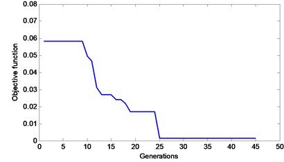
Fig. 11An objective function curve of the AFSA with visual-step change strategy for Case 2

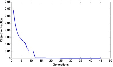
Fig. 12An objective function curve of the MSAFSA for Case 2

In general, measurement error will affect the credibility of experimental data. Here, the frequencies with 0.15 % error and the mode shapes with 3 % error are considered in this case. The IMSEDRI is used to identify suspected damage elements. The identification results of IMSEDRI with measurement error are depicted in Fig. 13. Here, we still select the highest five elements as suspected damage elements. Thus, the elements 7, 9, 27, 28 and 30 are picked out. The measurement error will also affect the identification results of the AFSAs. The basic AFSA, the AFSA with visual-step change strategy and the MSAFSA are used to assess the damage severity of the suspected damage elements. They only need to assess the damage severity of the suspected elements 7, 9, 27, 28 and 30. The calculation results are listed in Tables 11-13. From Table 11, we can find that the identification result of the basic AFSA isn’t very good. From Table 12, we can observe that the AFSA with visual-step change strategy can approximately find the true damage elements, but the average convergence speed isn’t very quick. From Table 13, we can observe that the MSAFSA can approximately find the true damage elements and improve the convergence speed. Therefore, the identification results of the MSAFSA are still superior to those of the basic AFSA and the AFSA with visual-step change strategy.

Fig. 13Damage identification results of the IMSEDRI with measurement error for Case 2

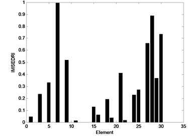
Table 11Quantitative results of 10 run with measurement error using the basic AFSA for Case 2

No.	Elements and damage					Iteration number
No.	7	9	27	28	30	Iteration number
1	0.1800	0.1700	0	0.2000	0	46
2	0.0100	0.1700	0	0.2100	0	58
3	0.5200	0.1700	0	0.1700	0	41
4	0.1800	0.1700	0	0.2000	0	30
5	0.1800	0.1700	0	0.2000	0	47
6	0.1800	0.1700	0	0.2000	0	55
7	0.4800	0.1300	0	0.2100	0	56
8	0.5300	0.1700	0	0.1600	0	54
9	0.5300	0.1700	0	0.1600	0	62
10	0.5300	0.1700	0	0.1600	0	45
Average	0.332	0.166	0	0.187	0	49.4

Table 12Quantitative results of 10 run with measurement error using the AFSA with visual-step change strategy for Case 2

No.	Elements and damage					Iteration number
No.	7	9	27	28	30	Iteration number
1	0.1900	0.1800	0	0.1900	0	25
2	0.1800	0.1700	0	0.2000	0	31
3	0	0.1900	0	0	0	28
4	0.5300	0.1700	0	0.1600	0	41
5	0.1800	0.1700	0	0.2000	0	35
6	0.5300	0.1700	0	0.1600	0	38
7	0.1800	0.1700	0	0.2000	0	29
8	0.0100	0.1700	0	0.2100	0	26
9	0.1800	0.1700	0	0.2000	0	32
10	0.1800	0.1700	0	0.2000	0	25
Average	0.216	0.173	0	0.172	0	31

From the two cases, we can find that the proposed two-stage method can detect structural damage with good accuracy. First, the IMSEDRI can approximately identify suspected damage elements. Then, the MSAFSA can calculate the damage extent of the suspected damage elements. Moreover, the proposed MSAFSA is superior to both the basic AFSA and the AFSA with visual-step change strategy.

In general, it is difficult for a single AFSA to identify structural multiple damage problem. To this problem, if the identification precision of damage extent is 1 %, we need to find the optimal solution from 101³⁰ $\approx$ 1.3478×10⁶⁰ different kinds of selection. However, the proposed two-stage method can efficiently reduce the search space. For example, in case 1, we have identified 5 suspected damage elements in the 30 elements by using the IMSEDRI. Thus, we just need to find the optimal solution from 101⁵ $\approx$ 1.051×10¹⁰ different kinds of selection. Actually, the average iteration number of the MSAFSA is 100×27.6 $=$ 2760. Therefore, the two-stage method is of better convergence and higher search efficiency.

Table 13Quantitative results of 10 run with measurement error using the MSAFSA for Case 2

No.	Elements and damage					Iteration number
No.	7	9	27	28	30	Iteration number
1	0.0100	0.1700	0	0.2100	0	27
2	0.1900	0.1700	0	0.2000	0	7
3	0.1800	0.1700	0	0.2000	0	13
4	0.1900	0.1700	0	0.2000	0	23
5	0.1600	0.1700	0	0.2000	0	8
6	0.1900	0.1700	0	0.2000	0	10
7	0.2200	0.1700	0	0.2000	0	7
8	0.2300	0.1700	0	0.2000	0	8
9	0.1600	0.1700	0	0.2000	0	6
10	0.2300	0.1700	0	0.2000	0	15
Average	0.176	0.17	0	0.201	0	12.4

7. Conclusions

This study has applied a two-stage damage identification method to diagnose structural damages and a novel AFSA has been developed. Subsequently, the results from a simulated structure model have been used to verify the effectiveness of the two-stage method and the MSAFSA. The process of applying the two-stage method and MSAFSA is also been described. First, the improved modal strain energy dissipation ration index is used to preliminarily identify the suspected damage elements. Then, the micro-search artificial fish swarm algorithm is utilized to find the damage extent of the suspected damage elements. The main conclusions are: Eq. (1) The two-stage method based on the IMSEDRI and MSAFSA can accurately and clearly locate damages and has the potential to quantify the degree of damage. Eq. (2) The MSAFSA can perform well under the condition of small damages and their performance is robust even under the interference of measurement error. Therefore, the MSAFSA is more effective and superior than both the basic AFSA and the AFSA with visual-step change strategy.

References

Cawley P., Adams R. D. The location of defects in structures from measurements of natural frequencies. Journal of Strain Analysis, Vol. 14, Issue 2, 1979, p. 49-57.

Publisher
Salawu O. S. Detection of structural damage through changes in frequency: a review. Engineering Structures, Vol. 19, Issue 9, 1997, p. 718-723.

Publisher
Chaudhari T. D., Maiti S. K. A study of vibration of geometrically segmented beams with and without crack. International Journal of Solids and Structures, Vol. 37, Issue 5, 2000, p. 760-779.

Publisher
Chinchalkar S. Determination of crack location in beams using natural frequencies. Journal of Sound and Vibration, Vol. 247, 2001, p. 417-429.

Publisher
Zhang Z., Shankar K., Morozov E. V., Tahtali M. Vibration-based delamination detection in composite beams through frequency changes. Journal of Vibration and Control, Vol. 22, Issue 2, 2014, p. 496-512.

Publisher
Law S. S., Shi Z. Y., Zhang L. M. Structural damage detection from incomplete and noisy modal data. ASCE Journal of Engineering Mechanics, Vol. 124, Issue 11, 1998, p. 1280-1288.

Publisher
Shi Z. Y., Law S. S., Zhang L. M. Optimum sensors placement for structural damage detection. ASCE Journal of Engineering Mechanics, Vol. 126, Issue 11, 2000, p. 1173-1179.

Publisher
Guo H., Zhang L. A weighted balance evidence theory for structural multiple damage localization. Computer Methods in Applied Mechanics and Engineering, Vol. 195, Issues 44-47, 2006, p. 6225-6238.

Publisher
Allemang R. J., Brown D. L. A correlation coefficient for modal vector analysis. 1st International Modal Analysis Conference, 1982, p. 110-116.

Search CrossRef
Pindey A. K., Biswas M. Experimental verification of flexibility difference method for locating damage in structures. Journal of Sound and Vibration, Vol. 184, Issue 2, 1995, p. 311-328.

Publisher
Venkatappa S. G. Damage Detection using Vibration Measurement. Master of Science Thesis, West Virginia University, 1997.

Search CrossRef
Stubbs N., Kim J. T., Farrar C. R. Field verification of a nondestructive damage localization and severity estimation algorithm. Proceedings of IMAC, Connecticut USA, Society of Experimental Mechanics, 1995, p. 210-218.

Search CrossRef
Hu H., Wu C. Development of scanning damage index for the damage detection of plate structures using modal strain energy method. Mechanical Systems and Signal Processing, Vol. 23, Issue 2, 2009, p. 274-287.

Publisher
Shi Z. Y., Law S. S., Zhang L. M. Structural damage localization from modal strain energy change. Journal of Sound and Vibration, Vol. 218, Issue 5, 1998, p. 825-844.

Publisher
Sazonov E., Klinkhachorn P. Optimal spatial sampling interval for damage detection by curvature or strain energy mode shapes. Journal of Sound and Vibration, Vol. 285, Issue 4-5, 2005, p. 783-801.

Publisher
Liu H., Qu W. L., Yuan R. Z. Structural damage detection method based on the theory of dissipation ratio of modal strain energy. Journal of Vibration and Shock, Vol. 23, Issue 2, 2004, p. 118-121, (in Chinese).

Search CrossRef
Li X., Shao Z., Qian J. An optimizing method base on autonomous animates: fish swarm algorithm. Systems Engineering Theory and Practice, Vol. 22, Issue 11, 2002, p. 32-38.

Search CrossRef
Azad M. A., Rocha A. M. A. C., Fernandes. E. G. P. Improved binary artificial fish swarm algorithm for the 0-1 multidimensional knapsack problems. Swarm and Evolutionary Computation, Vol. 14, 2014, p. 66-75.

Publisher
Tsai H. C., Lin Y. H. Modification of the fish swarm algorithm with particle swarm optimization formulation and communication behavior. Applied Soft Computing, Vol. 11, Issue 8, 2011, p. 5367-5374.

Publisher
Zhou Z. B. Principle of Least Energy Dissipation and Its Application. 1st Ed., Beijing, China Science Press, 2001.

Search CrossRef
Seyedpoor S. M. A two-stage method for structural damage detection using a modal strain energy based index and particle swarm optimization. International Journal of Non-linear Mechanics, Vol. 47, Issue 1, 2012, p. 1-8.

Publisher

Cited by

Reactive Power Optimization Using New Enhanced Whale Optimization Algorithm

Imran Rahman | Junita Mohamad-Saleh | Noorazliza Sulaiman

(2022)

Damage Identification of Bridge Structures Considering Temperature Variations-Based SVM and MFO

Minshui Huang | Yongzhi Lei | Xifan Li | Jianfeng Gu

(2021)

About this article

Received

02 August 2016

Accepted

13 February 2017

Published

15 August 2017

SUBJECTS

Fault diagnosis based on vibration signal analysis

DOI

https://doi.org/10.21595/jve.2017.17503

Keywords

damage identification

artificial fish swarm algorithm

modal strain energy

visual distance

step length

Acknowledgements

This work was supported by the National Natural Science Foundation of China (Grant No. 51468058, 51578094), and the Fundamental Research Funds for the Central Universities (Grant No. 106112014CDJZR200011).

This is an open access article distributed under the Creative Commons Attribution License, which permits unrestricted use, distribution, and reproduction in any medium, provided the original work is properly cited.

Previous article in issue Previous Next article in issue Next

Research article

2023 10 20

Damage detection in variable temperature conditions using artificial intelligence

Alexandra-Teodora Aman, Cristian Tufisi, Gilbert-Rainer Gillich, Tiberiu Manescu

Research article

2020 04 02

Damage detection in a fixed-fixed beam using natural frequency changes

Muhammad Wasif Khan, Naveed Akmal Din, Rizwan Ul Haq

Research article

2019 11 15

Damage identification research on beam structures by integrating multiple modal parameters

Jingbo Duan, Wenjie Wang, Weiyong Zhou

Research article

2019 02 15

Sensitivity analyses of resonant frequencies and modal strain energy of damaged beams by perturbation method

G. Chen, P. P. Gong, P. Liang

H. Guo, “Structural multi-damage identification based on strain energy and micro-search artificial fish swarm algorithm,” Journal of Vibroengineering, Vol. 19, No. 5, pp. 3255–3270, Aug. 2017, https://doi.org/10.21595/jve.2017.17503

Copy Extrica

Copied to clipboard!

TY  - JOUR
DO  - 10.21595/jve.2017.17503
UR  - https://doi.org/10.21595/jve.2017.17503
TI  - Structural multi-damage identification based on strain energy and micro-search artificial fish swarm algorithm
T2  - Journal of Vibroengineering
AU  - Guo, Huiyong
PY  - 2017
DA  - 2017/08/15
PB  - JVE International Ltd.
SP  - 3255-3270
IS  - 5
VL  - 19
SN  - 1392-8716
ER  - 

Copy Ris

Copied to clipboard!

@article{Guo_2017,
	doi = {10.21595/jve.2017.17503},
	url = {https://doi.org/10.21595/jve.2017.17503},
	year = 2017,
	month = {aug},
	publisher = {{JVE} International Ltd.},
	volume = {19},
	number = {5},
	pages = {3255--3270},
	author = {Huiyong Guo},
	title = {Structural multi-damage identification based on strain energy and micro-search artificial fish swarm algorithm},
	journal = {Journal of Vibroengineering}
}

Copy Bibtex

Copied to clipboard!

[1]H. Guo, “Structural multi-damage identification based on strain energy and micro-search artificial fish swarm algorithm,” Journal of Vibroengineering, vol. 19, no. 5, pp. 3255–3270, Aug. 2017, doi: 10.21595/jve.2017.17503.

Copy IEEE

Copied to clipboard!

Guo, Huiyong. “Structural Multi-Damage Identification Based on Strain Energy and Micro-Search Artificial Fish Swarm Algorithm.” Journal of Vibroengineering 19, no. 5 (August 15, 2017): 3255–70. https://doi.org/10.21595/jve.2017.17503.

Copy Chicago

Copied to clipboard!

Structural multi-damage identification based on strain energy and micro-search artificial fish swarm algorithm

Abstract

1. Introduction

2. Improved modal strain energy dissipation ration index

3. Artificial fish swarm algorithm

3.1. Foraging behavior

3.2. Swarming behavior

3.3. Following behavior

3.4. Random behavior

4. Micro-search artificial fish swarm algorithm

4.1. Visual-step change strategy

4.2. Micro-search strategy

4.3. Two termination criteria.

5. Damage identification based on artificial fish swarm algorithm

6. Numerical examples

6.1. Case 1

6.2. Case 2

7. Conclusions

References

Cited by

About this article

Related Articles