Axial dynamic load identification of hydraulic turbine based on Chebyshev orthogonal polynomial approximation

Song, Zhiqiang; Liu, Yunhe

doi:10.21595/jve.2016.17535

Journal of Vibroengineering

Browse Journal

Submit article

Published: 15 February 2017

Check for updates

Axial dynamic load identification of hydraulic turbine based on Chebyshev orthogonal polynomial approximation

Zhiqiang Song¹

Yunhe Liu²

^{1, 2}State Key Laboratory Base of Eco-hydraulic Engineering in Arid Area, Xi’an University of Technology, Xi’an, China

Corresponding Author:

Zhiqiang Song

Cite the article Download PDF

Downloads 1544

Abstract

An analysis method is proposed to identify axial dynamic loads acting on the Francis turbine based on Chebyshev orthogonal polynomial expansion theory. Dynamic loads are expressed as functions of time and polynomial coefficients. The dynamic load identification model is constructed through discretized integral convolution of the loads, such as the Duhamel integral. However, the discretized numerical integral has a time-cumulative error problem that decreases the recognition accuracy of the dynamic load. Compared with the traditional method, the algorithm proposed in this paper constructs the relationship between the modal displacement and force using polynomial orthogonality and derivative relation between displacement and velocity or acceleration. The new method could avoid the Duhamel integral and time-cumulative error problem. This algorithm not only requires less measuring point information, but is also highly efficient. Compared with genetic algorithm identification, orthogonal polynomial algorithm is not easy falling into local convergence, and does not require multiple repetitions positive analysis trial to evaluate individual fitness value. Numerical simulations demonstrate that the identification and assessment of dynamic loads are effective and consistent when the proposed method is used.

1. Introduction

Nowadays, dynamic loads play an important role in many practical engineering problems [1-6]. The dynamic load must be known when various methods are used in dynamics analysis to ensure the reliability and safety of engineering structures. However, in some cases, such as axial dynamic loads of hydro-generator turbines, it is difficult to directly measure the dynamic loads due to limits of technical or economic conditions. However, the dynamic response is easily measured, which leads to the development of the theory of load identification.

There are two main identification methods: frequency-domain technique and time-domain technique [7, 8]. The frequency-domain technique determines the load spectrums by the frequency response functions and the response spectrums measured, or calculates the modal forces in modal space through coordinate changes [9-12]. Compared with frequency-domain identification, the time-domain technique has good accuracy and clear physical meaning. H. Ocry, H. Glaser [13] determined the load firstly using the time-domain technique through modal coordinates changed in 1985. Recently, the time-domain technique has been greatly developed.

In practical engineering problems, the physical, geometrical, and boundary characteristics are generally uncertain due to errors in manufacture and installation, as well as complex working conditions. This prevents traditional identification methods from achieving good accuracy. Therefore, developing an efficient method to estimate the load of the rotating machinery has theoretical value and wide engineering significance. R. Tiwari and V. C. simultaneously identified the residual unbalanced load and bearing dynamic parameters [14]. Chu and Zhang proposed an improved time-domain identification method through the Duhamel integral; Zhang also identified a two-dimensional distributed dynamic load through the Duhamel integral, and pointed out that the Duhamel integral has a time-cumulative error effect [15-17]. Some researchers determined a hydro-electric unit dynamic load through genetic algorithm or heuristic search algorithm according to the measured displacement [18-21]. The two algorithms identification processes require a number of trials to obtain better population reproduction. Furthermore, the calculation efficiency is poor. Liu et al. identified structures for dynamic loads through various methods, such as the Galerkin method which weighed the total least squares method; Gegenbauer polynomial approximation method; second-order Taylor-Series expansion method, SVM regression approach; and virtual work principle [22-27]. Some scholars are committed to solve the impact of noise during the identification by proposing a method that integrates denoising, correction, regularization preconditioned iteration method, and Kalman filter or Monte Carlo filter method [28-30].

For a water turbine generator set, the distances of upper and lower guide bearings are asymmetrical relative to the rotor. The rotor rotates forming arcuate cyclotron, has not only horizontal displacement, but also vertical displacement (Angular displacement). That is the gyroscopic effect. Usually, modal uncoupling of gyroscopic systems is difficult to carry out without additional assumptions and simplifications. However, this study aims to identify the unknown desired axial dynamic load of a rotor bearing system based on Chebyshev orthogonal polynomial theory, instead of radial dynamic loads. This study constructs the unit shaft system and pier coupling vibration model consider vertical freedom only. The gyroscopic effect is not considered during the modal decoupling.

This paper is organized as follows. Section 2 introduces the basic theories of the Chebyshev Polynomials and determines the algorithm of the dynamic load on the basis of orthogonal polynomial expansion. Compared with other research that used the traditional method, this study constructs the relationship between the modal displacement and force using the Chebyshev Polynomial orthogonality instead of the Duhamel integral. This method could avoid a Duhamel integral time-cumulative error effect. Moreover, Section 3 adopts the proposed method to solve the determined equation and identify the unknown desired dynamic load through numerical examples. Finally, Section 4 provides the conclusion.

2. Dynamic load identification based on orthogonal polynomial decomposition

Generalized Chebyshev orthogonal polynomials can be used to approximate any continuous single-valued function. As long as the order is reasonable and sufficient, it is better to identify the time-varying dynamic load [17].

The fitting form of the generalized time interval [0, $S$ ] is as follows:

1

f (t) = \sum_{j = 0}^{\infty} a_{j} T_{j} (t),

2

\{\begin{array}{l} T_{0} (t) = \frac{1}{\sqrt{π}}, \\ T_{1} (t) = \frac{\sqrt{2}}{\sqrt{π}} (\frac{2}{s} \cdot t - 1), \\ T_{2} (t) = \frac{\sqrt{2}}{\sqrt{π}} (2 {(\frac{2}{s} \cdot t - 1)}^{2} - 1) . \\ \dots \end{array}

The recursive formula is shown below:

3

T_{j + 1} (t) = 2 (\frac{2}{s} \cdot t - 1) \cdot T_{j} (t) - T_{j - 1} (t), j \geq 2 .

The Chebyshev orthogonal polynomial coefficients $a_{j}$ are determined by:

4

a_{j} = \int_{0}^{s} h (t) \cdot f (t) T_{j} (t) d t,

where, $h (t)$ is weight function.

The system motion equation for an arbitrary $n$ order multi-degrees is:

5

[M] \{\begin{matrix} {\ddot{u}}_{1} (t) \\ ⋮ \\ {\ddot{u}}_{k} (t) \\ ⋮ \\ {\ddot{u}}_{n} (t) \end{matrix}\} + [C] \{\begin{matrix} {\dot{u}}_{1} (t) \\ ⋮ \\ {\dot{u}}_{k} (t) \\ ⋮ \\ {\dot{u}}_{n} (t) \end{matrix}\} + [K] \{\begin{matrix} u_{1} (t) \\ ⋮ \\ u_{k} (t) \\ ⋮ \\ u_{n} (t) \end{matrix}\} = \{\begin{matrix} 0 \\ ⋮ \\ F_{m} (t) \\ ⋮ \\ 0 \end{matrix}\},

where [ $M$ ], [ $C$ ], and [ $K$ ] are the mass matrix, damping matrix, and stiffness matrix of the system; ${\ddot{u}}_{k} (t)$ , ${\dot{u}}_{k} (t)$ , $u_{k} (t)$ are acceleration, velocity and displacement of the measuring point. $F_{m} (t)$ is the load on node $m$ , which is waited to be identified.

Assuming that damping is proportional damping, modal coordinate transformation is introduced:

6

\{u (t)\} = [Φ] \{y (t)\} = [\begin{matrix} ϕ_{11} & ϕ_{1 i} & \dots & ϕ_{1 n} \\ ϕ_{k 1} & ϕ_{k i} & \dots & ϕ_{k n} \\ ⋮ & ⋮ & ⋱ & ⋮ \\ ϕ_{n 1} & ϕ_{n i} & \dots & ϕ_{n n} \end{matrix}] \{y (t)\},

where, $[Φ]$ is principal modal matrix, $y (t)$ is the $i$ th modal displacement:

7

[M] [Φ] \{\ddot{y} (t)\} + [C] [Φ] \{\dot{y} (t)\} + [K] [Φ] \{y (t)\} = \{F (t)\} .

Left-multiplied ${[Φ]}^{T}$ , the system can be decoupled into $n$ single degree of freedom systems according to modal shape orthogonality:

8

M_{i}^{*} {\ddot{y}}_{i} (t) + C_{i}^{*} {\dot{y}}_{i} (t) + K_{i}^{*} y_{i} (t) = ϕ_{m i} F_{m} (t) = f_{i} (t) \begin{array}{l} , & i = 1,2, \dots n \end{array},

where $M_{i}^{*}$ , $C_{i}^{*}$ , $K_{i}^{*}$ and $f_{i} (t)$ are the modal mass, modal damping, modal stiffness, and modal force in the $i$ th order; and ${\ddot{y}}_{i} (t)$ , ${\dot{y}}_{i} (t)$ , $y_{i} (t)$ are modal acceleration, velocity, and displacement in the $i$ th order.

Chebyshev orthogonal polynomial expansion of the $i$ th order modal force $f_{i} (t)$ is:

9

f_{i} (t) = \sum_{j = 0}^{\infty} a_{i j} T_{j} (t) .

According to Duhamel integral:

10

y_{i} (t) = \frac{1}{M_{i}^{*} ω_{D i}} \int_{0}^{t} f_{i} (τ) e^{- ξ_{i} ω_{i} (t - τ)} s i n [ω_{D i} (t - τ)] d τ

= \frac{\sum_{j = 0}^{\infty} a_{i j}}{M_{i}^{*} ω_{D i}} \int_{0}^{t} T_{j} (τ) e^{- ξ_{i} ω_{i} (t - τ)} s i n [ω_{D i} (t - τ)] d τ = [\begin{array}{l} d_{i 0} & d_{i j} & \dots & d_{i \infty} \end{array}] \{\begin{matrix} a_{i 0} \\ a_{i j} \\ ⋮ \\ a_{i \infty} \end{matrix}\},

where, $C_{i}^{*} = 2 ξ_{i} ω_{i} {M_{i}}^{*}$ , $ω_{D i} = ω_{i} \sqrt{1 - ξ_{i}^{2}}$ , $d_{i j} = \frac{1}{M_{i}^{*} ω_{D i}} \int_{0}^{t} T_{j} (τ) e^{- ξ_{i} ω_{i} (t - τ)} s i n [ω_{D i} (t - τ)] d τ$ .

Substitute Eq. (10) into Eq. (6):

11

\{u_{k}\} = [\begin{array}{l} ϕ_{k 1} \cdot [D_{1}] & ϕ_{k i} \cdot [D_{i}] & \dots & ϕ_{k n} \cdot [D_{n}] \end{array}] \{\begin{matrix} \{A_{1}\} \\ \{A_{i}\} \\ ⋮ \\ \{A_{n}\} \end{matrix}\},

where, $[D_{i}] = [\begin{array}{l} d_{i 0} & d_{i j} & \dots & d_{i \infty} \end{array}]$ , $\{A_{i}\} = {\{\begin{array}{l} a_{i 0} & a_{i j} & \dots & a_{i \infty} \end{array}\}}^{T}$ .

It is assumed that each order modal force needs $J$ terms expression to satisfy accuracy requirement. The system has $n$ order modals. The number of coefficients to be identified is $J^{*} n$ . Dispersing the measuring point displacement at different $J^{*} n$ times in the calculation interval could obtain $J^{*} n$ equations. All the orthogonal polynomials coefficients could be obtained by solving the equations. Subsequently, the dynamic load could be identified according to Eqs. (8) and (9).

The method above constructs the relationship between modal displacement and modal force by Duhamel integral in modal space. Eq. (10) shows that integral upper limit of the Duhamel integral is calculated instantaneously. In others words, the Duhamel integral calculation must be performed at each discrete time; the integral results are different at different times. Thus, the method above not only requires a large amount of computation, but also has a time-accumulation error problem.

The problem could be improved by decreasing time step and increasing orthogonal polynomials order number. However, it needs more calculation and require more measuring point information.

In this study, a new algorithm is proposed to solve the problem. The algorithm constructs the relationship between modal displacement and modal force by polynomial orthogonality and derivative relation between the displacement and velocity or acceleration. This method could avoid Duhamel integral and integral time-cumulative error problem as well as increase identification accuracy.

The orthogonal polynomial expansions of the $i$ th order modal force, displacement, velocity and acceleration are as follows:

12

\{\begin{array}{l} f_{i} (t) = \sum_{j = 0}^{\infty} a_{i j} T_{j} (t), \\ y_{i} (t) = \sum_{j = 0}^{\infty} b_{i j} T_{j} (t), \\ {\dot{y}}_{i} (t) = \sum_{j = 0}^{\infty} {b^{'}}_{i j} T_{j} (t), \\ {\ddot{y}}_{i} (t) = \sum_{j = 0}^{\infty} {b^{''}}_{i j} T_{j} (t) . \end{array}

Substitute Eq. (12) into Eq. (8):

13

M_{i}^{*} \sum_{j = 0}^{\infty} b_{i j}^{''} T_{j} (t) + C_{i}^{*} \sum_{j = 0}^{\infty} b_{i j}^{'} T_{j} (t) + K_{i}^{*} \sum_{j = 0}^{\infty} b_{i j} T_{j} (t) = \sum_{j = 0}^{\infty} a_{i j} T_{j} (t) .

Assuming that the calculation of time interval is [0, $T$ ], multiply $T_{g} (t) h (t)$ on both sides of Eq. (13) and integral in interval [0, $T$ ]. According to polynomials weighted orthogonality:

14

M_{i}^{*} b_{i g}^{''} + C_{i}^{*} b_{i g}^{'} + K_{i}^{*} b_{i g} = a_{i g} \begin{array}{l} , & g = 0,1, 2, \dots \infty \end{array},

where $b_{i g}^{''}$ , $b_{i g}^{'}$ and $b_{i g}$ are determined by:

15

\{\begin{array}{l} b_{i g}^{''} = \int_{0}^{T} {\ddot{y}}_{i} (t) \cdot T_{g} (t) \cdot h (t) d t, \\ b_{i g}^{'} = \int_{0}^{T} {\dot{y}}_{i} (t) \cdot T_{g} (t) \cdot h (t) d t, \\ b_{i g} = \int_{0}^{T} y_{i} (t) \cdot T_{g} (t) \cdot h (t) d t . \end{array}

According to the derivative relation between the displacement and acceleration or velocity:

16

\{\begin{array}{l} {\ddot{y}}_{i} (t) = \sum_{j = 0}^{\infty} b_{i j} {\ddot{T}}_{j} (t), \\ {\dot{y}}_{i} (t) = \sum_{j = 0}^{\infty} b_{i j} {\dot{T}}_{j} (t) . \end{array}

Substitute Eq. (16) into Eq. (15):

17

\{\begin{array}{l} b_{i g}^{''} = \int_{0}^{T} \sum_{j = 0}^{\infty} b_{i j} {\ddot{T}}_{j} (t) \cdot T_{g} (t) \cdot h (t) d t = \sum_{j = 0}^{\infty} p_{j g}^{i} b_{i j}, \\ b_{i g}^{'} = \int_{0}^{T} \sum_{j = 0}^{\infty} b_{i j} {\dot{T}}_{j} (t) \cdot T_{g} (t) \cdot h (t) d t = \sum_{j = 0}^{\infty} q_{j g}^{i} b_{i j}, \end{array}

18

\{\begin{array}{l} p_{j g}^{i} = \int_{0}^{T} {\ddot{T}}_{j} (t) \cdot T_{g} (t) \cdot h (t) d t, \\ q_{j g}^{i} = \int_{0}^{T} {\dot{T}}_{j} (t) \cdot T_{g} (t) \cdot h (t) d t . \end{array}

Substitute Eq. (17) into Eq. (14). The new relationship is constructed between displacement and force in mode space:

19

(M_{i}^{*} [I] [P^{i}] + C_{i}^{*} [I] [Q^{i}] + K_{i}^{*} [I]) \{b_{i}\} = \{a_{i}\}, \begin{array}{l} i = 1,2, \dots, n \end{array},

where [ $I$ ] is the unit matrix, and:

[P^{i}] = [\begin{matrix} p_{00}^{i} & p_{01}^{i} & \dots & p_{0 \infty}^{i} \\ p_{10}^{i} & p_{11}^{i} & \dots & p_{1 \infty}^{i} \\ ⋮ & ⋮ & ⋮ & ⋮ \\ p_{\infty 0}^{i} & p_{\infty 1}^{i} & \dots & p_{\infty \infty}^{i} \end{matrix}], [Q^{i}] = [\begin{matrix} q_{00}^{i} & q_{01}^{i} & \dots & q_{0 \infty}^{i} \\ q_{10}^{i} & q_{11}^{i} & \dots & q_{1 \infty}^{i} \\ ⋮ & ⋮ & ⋮ & ⋮ \\ q_{\infty 0}^{i} & q_{\infty 1}^{i} & \dots & q_{\infty \infty}^{i} \end{matrix}],

where $\{b_{i}\}$ , $\{a_{i}\}$ are the coefficient vectors of the modal displacement and force in $i$ th order.

The measuring point time domain displacement could be expressed by principal modal matrix and modal displacement. The orthogonal polynomial coefficients could be solved by constructing equations through dispersing the measuring point displacement at different times. Consequently, dynamic load identification could be performed.

The algorithm proposed in this paper constructs the relationship between modal displacement and force according to polynomial orthogonality and derivative relation between the displacement and velocity or acceleration. This method could avoid Duhamel integral and increase identification accuracy. Although each element in [ $P$ ] or [ $Q$ ] matrices must be calculated during the integration, the integral upper limit is the same. That is, the integral result remains constant at different times. Implementing integral operation at each discrete time becomes unnecessary. The algorithm increases recognition accuracy and improves calculation efficiency.

The modal mass, stiffness, frequency and shape must be known during load identification. The frequency and mode shape could be easily obtained through modal analysis. The modal mass could be obtained through Eq. (20) as demonstrated in an earlier study [31]:

20

M_{i}^{*} = \frac{2.0 E_{i}}{{ω_{i}}^{2}},

where $E_{i}$ is the $i$ th order modal kinetic energy. Furthermore, the modal stiffness and damping could be deduced.

3. Numerical examples

This study used a practical hydro-generator unit as example. A hydro-generator shaft system and pier coupling vertical vibration model was constructed. The pier was regarded as a rigid foundation. The thrust bearing and frame centrosome was regarded as a spring element. The large shaft was simplified as a non-mass elastic beam. Its mass was distributed into three nodes, which represent the exciter, rotor and runner. The rotor arm was simplified as a non-mass elastic rod. The average quality was assigned to the edge of the rotor bracket and frame centrosome. The mass spring system model is shown in Fig. 1. Moreover, the values and meanings of all parameters are shown in Table 1 [5-6].

Fig. 1Vertical vibration simplified model of the hydro-generator

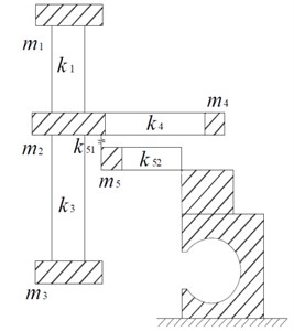
The total stiffness matrix of the system is:

21

[K] = (\begin{matrix} k_{1} & - k_{1} & 0 & 0 & 0 \\ - k_{1} & k_{1} + k_{3} + k_{4} + k_{51} & - k_{3} & - k_{4} & - k_{51} \\ 0 & - k_{3} & k_{3} & 0 & 0 \\ 0 & - k_{4} & 0 & k_{4} & 0 \\ 0 & - k_{51} & 0 & 0 & k_{51} + k_{52} \end{matrix}) .

Table 1Values and meanings of the parameters of the simplified vertical vibration model

	Equivalent value	Equivalent meaning
$m_{1}$	8.28×10⁴kg	Exciter mass+1/2 shaft segment mass from top to rotor support frame
$m_{2}$	1.042×10⁶ kg	Rotor support frame centrosome mass +1/2 total arms mass +1/2 total shaft mass
$m_{3}$	3.29×10⁵ kg	Runner mass+ water addition quality+1/2 shaft segment mass from rotor support frame to runner
$m_{4}$	9×10⁵ kg	Magnetic yoke and magnetic pole mass at rotor edge
$m_{5}$	1.2×10⁵ kg	Under frame centrosome mass+1/2 total under frame arms mass
$k_{1}$	7.25×10¹⁰(N/m)	tensile stiffness of the shaft segment
$k_{3}$	5.72×10¹⁰ (N/m)	tensile stiffness of the shaft segment
$k_{4}$	2.32×10¹⁰ (N/m)	Total vertical stiffness of rotor frame arms
$k_{51}$	2.20×10¹² (N/m)	thrust bearing equivalent vertical stiffness between m₂ andm₅
$k_{52}$	9.41×10⁹ (N/m)	Total vertical stiffness of under frame arms

The lumped mass matrix is:

22

[M] = d i a g \{m_{1}, m_{2}, m_{3}, m_{4}, m_{5}\} .

The damping matrix was acquired using the Rayleigh proportional damping model. The damping ratio $ξ$ was 0.05. The first and second order circular frequencies were used to calculate the coefficients of mass matrix and stiffness matrix in Eq. (23):

23

[C] = α [M] + β [K]

where $α = 2 ξ ω_{1} ω_{2} / (ω_{1} + ω_{2})$ , $β = 2 ξ / (ω_{1} + ω_{2})$ .

The modal parameters obtained through model analysis are shown in Table 2.

Table 2Modal parameters of the vertical vibration model

Modal order	Parameter
Modal order	Circular frequency (Hz)	Modal mass (Kg)	Modal stiffness (N/m)	Modal damping (N·s/m)	Modal shape (−)
1	59.75	2.08×10⁶	7.42×10⁹	1.24×10⁷	[0.87,0.86,0.88,1,0.86]^T
2	204.24	1.59×10⁶	6.66×10¹⁰	3.26×10⁷	[−0.65,−0.62,−0.81,1,−0.62]^T
3	474.47	4.45×10⁵	1.00×10¹¹	3.99×10⁷	[−0.40,−0.29,1,0.04,−0.30]^T
4	972.32	9.01×10⁴	8.51×10¹⁰	3.27×10⁷	[1,−0.08,0.02,0.002,−0.08]^T
5	4531.06	1.34×10⁵	2.73×10¹²	1.04×10⁹	[0.005,−0.12,0.001,0.0001,1]^T

Construct axial hydro-thrust for Francis turbine according to the literature [19]:

24

F = 142.7 \times 1 0^{3} c o s (2 π \times 0.29 t + 1.04) + 438.9 \times 1 0^{3} c o s (2 π \times 1.25 t + 4.39)

- 287.4 \times 1 0^{3} c o s (2 π \times 2.5 t + 5.07) + 489.7 \times 1 0^{3} c o s (2 π \times 8.75 t + 1.43) .

The dynamic load above was applied to the runner node, which is node 3. The under-frame centrosome displacement could be obtained through calculation. The response and additional 10 % random noise was regarded as the known measuring point displacement. The axial hydro-thrust was identified using the orthogonal polynomial decomposition algorithm.

The identification used two cases. Case 1 constructed the relationship between modal displacement and force through the Duhamel integral. Case 2 constructed the relationship according to the polynomial orthogonality and derivative relationship between displacement and velocity or acceleration as mentioned above. The identified dynamic loads of the two cases are shown in Fig. 2 and Fig. 3. The figures show that the algorithm proposed in this paper avoids Duhamel integral and improves time-cumulative error effect. The integral result of the [ $P$ ] and [ $Q$ ] matrices remain constant at different times. Implementing integral operation at each discrete time has become unnecessary. The algorithm increases recognition accuracy and improves calculation efficiency.

Fig. 2Identification result of Case 1

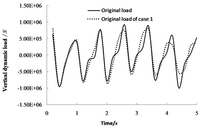
Fig. 3Identification result of Case 2

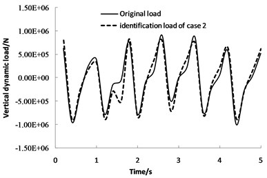
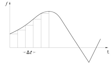
Fig. 4 shows relative instantaneous error and time-cumulative error of the two algorithms. The cumulative errors are sum of absolute value of the relative error in each calculation time. The cumulative error of the proposed method could converge at a certain time step. However, the cumulative error of the Duhamel integral method would diverge with time step. There are two kinds of factor which lead to the cumulative error. First, the discrete step could not be infinitely small because of the calculation efficiency. For example, in Fig. 5, the cumulative error is difference between the discrete summation and continuous integral. Second, the finite element load applying method could not be an ideal state step mutation. For instance, in Fig. 6, difference of the load applying methods also lead to a cumulative error.

Fig. 4Identification error of the two cases

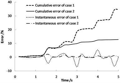
Fig. 5Cumulative error due to discretion

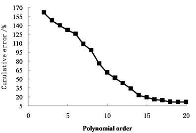
An empirical method in literature [32] could be used to determine the order number of the orthogonal polynomial. However, the formula mainly be applied to two-dimensional orthogonal polynomials for distributed dynamic load identification. For one-dimensional orthogonal polynomials, the cumulative error convergence trend chart with orthogonal polynomial order number could be used to determine the order number. Fig. 7 shows the curves of identification cumulative error with the orthogonal polynomials order number. The cumulative error decreases as the order increases. When the order number is up to 16, the error is convergent, and the result is credible.

The identified dynamic load was applied to the structure. The whole structure dynamic response can be obtained. Using the displacement response of node 5 multiplied by the stiffness of $k_{52}$ , the dynamic load transferred from the under frame and the pier could be obtained, that is, the vertical exciting load of the pier.

Fig. 6Cumulative error due to load handing method

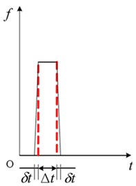
Fig. 7Cumulative error with polynomials order

4. Conclusions

An analysis method is proposed to identify dynamic loads based on Chebyshev orthogonal polynomial expansion theory. This algorithm not only requires less measuring point information, but is also highly efficient. Compared with genetic algorithm identification, orthogonal polynomial algorithm is not easy falling into local convergence, and does not require multiple repetitions positive analysis trial to evaluate individual fitness value.

The traditional dynamic load identification model is constructed through discretized integral convolution of the loads, such as the Duhamel integral. The discretized numerical integral has a time-cumulative error problem that decreases the recognition accuracy of the dynamic load. Compared with the traditional method, the algorithm proposed in this paper constructs the relationship between the modal displacement and force using polynomial orthogonality and derivative relation between displacement and velocity or acceleration. The new method could avoid the Duhamel integral and time-cumulative error problem. Performing an integral calculation for a coefficient matrix at each discrete time becomes unnecessary. The proposed algorithm has higher identification accuracy and efficiency than the traditional Duhamel integral algorithm.

References

Kashani Mir Tahmaseb, Jayasinghe Supun, Hashemi Seyed M. Dynamic finite element analysis of bearing-torsion coupled beams subjected to combined axial load and end moment. Shock and Vibration, Vol. 2015, 2015, p. 471270.

Publisher
Hadi Jalali Mohammad, Ghayour Mostafa, Ziaei-Rad Saeed, et al. Dynamic analysis of a high speed rotor-bearing system. Measurement, Vol. 54, 2014, p. 1-9.

Publisher
Si Xiaohui, Lu Wen Xiu, Chu Fuller Lateral vibration of hydroelectric generating set with different supporting condition of thrust pad. Shock and Vibration, Vol. 18, 2011, p. 317-331.

Publisher
Sun Wanquan, Huang Xionghui Identification of vibration transfer path for the coupled system of water turbine generator set and power house. Journal of Vibration and Shock, Vol. 33, Issue 6, 2014, p. 23-28.

Search CrossRef
Ma Zhenyue, Dong Yuxin Dynamics of Water Turbine Generator Set. Dalian University of Technology Press, Dalian, 2003.

Search CrossRef
Zhi Baoping, Ma Zhenyue, Wu Qianqian Study on transfer paths of vertical vibrations in the head cover system of turbine. Journal of Hydroelectric Engineering, Vol. 32, Issue 3, 2013, p. 241-245.

Search CrossRef
Xu Feng, Chen Huaihai, et al. Force identification for mechanical vibration state-of-the-art and prospect. China Mechanical Engineering, Vol. 13, Issue 6, 2002, p. 526-531.

Search CrossRef
Uhl T. The inverse identification problem and its technical application. Archive of Applied Mechanics, Vol. 77, Issue 5, 2007, p. 325-337.

Publisher
Hillary B., Ewins D. J. The use of strain Gauges in force determination and frequency response function measurements. Proceedings of the 2nd International Modal Analysis Conference, Florida, USA, 1984, p. 627-634.

Search CrossRef
Zhu Dechun, Zhang Fang, Jiang Jinhui Identification technology of dynamic load location. Journal of Vibration and Shock, Vol. 31, Issue 1, 2012, p. 20-23.

Search CrossRef
Thite A. N., Thompson D. J. The quantification of structure-borne transmission paths by inverse methods. Part1: Improved singular value rejection methods. Journal of Sound and Vibration, Vol. 264, Issue 2, 2003, p. 411-431.

Publisher
Liu Y., Shepared Jr. W. S. Dynamic force identification based on enhanced least squares and total least-squares schemes in the frequency domain. Journal of Sound and Vibration, Vol. 282, Issue 1, 2005, p. 37-60.

Publisher
Ory H., Glaser H., Holzdeppe D. The reconstruction of forcing function based on measured structural responses. Proceeding of 2nd International Symposium on Aeroelasticity and Structural Dynamics, Aachen, 1985.

Search CrossRef
Tiwari R., Chakravarthy V. Simultaneous identification of residual unbalances and bearing dynamic parameters from impulse responses of rotor-bearing systems. Mechanical Systems and Signal Processing, Vol. 20, 2006, p. 1590-1614.

Publisher
Chu Liangcheng, Qu Naisi, Wu Ruifeng Dynamic load identification in time domain. Chain Ocean Engineering, Vol. 5, Issue 3, 1991, p. 279-286.

Search CrossRef
Zhang Yunliang, Lin Gao, Wang Yongxue, et al. An improved method of dynamic load identification in time domain. Chinese Journal of Computational Mechanics, Vol. 21, Issue 2, 2004, p. 209-214.

Search CrossRef
Zhang Yongcheng A Time Domain Method on Two Dimensional Distributed Dynamic Load Identification. Nanjing University of Aeronautics and Astronautics, 2007.

Search CrossRef
Li Shouju, Liu Yingxi, Ren Mingfa, et al. Identification procedures of vibration loading parameters of hydraulic generator based on improved genetic algorithm. Engineering Mechanics, Vol. 20, Issue 5, 2003, p. 163-169.

Search CrossRef
Wang Haijun, Lian Jijian, Yang Min, et al. Identification of axial dynamic load of a Francis Turbine. Journal of Vibration and Shock, Vol. 26, Issue 4, 2007, p. 123-125.

Search CrossRef
Helio Fiori de Castro, Katia Lucchesi Cavalca, Lucas Ward Franco de Camargo, et al. Identification of unbalance forces by metaheuristic search algorithm. Mechanical Systems and Signal Processing, Vol. 24, 2010, p. 1785-1789.

Publisher
Chisari Corrado, Bedon Chiara, Amadio Claudio Dynamic and static identification of base-isolated bridges using genetic algorithms. Engineering Structures, Vol. 102, 2015, p. 80-92.

Publisher
Liu Jie, Meng Xianghua, Jiang Chao Time-domain Galerkin method for dynamic load identification. International Journal for Numerical Methods in Engineering, Vol. 105, Issue 6, 2016, p. 620-640.

Publisher
Jia You, Yang Zhichun, Guo Ning Random dynamic load identification based on error analysis and weighted total least squares method. Journal of Sound and Vibration, Vol. 358, Issue 12, 2015, p. 111-123.

Publisher
Liu Jie, Sun Xingsheng, Han Xu, et al. Dynamic load identification for stochastic structures based on Gegenbauer polynomial approximation and regularization method. Mechanical Systems and Signal Processing, Vol. 56, 2015, p. 35-54.

Publisher
Li Xiaowang, Deng Zhongmin Identification of dynamic loads based on second-order Taylor-Series expansion method. Shock and Vibration, Vol. 2016, 2016, p. 6461427.

Publisher
Mao Wentao, Hu Dike, Yan Guirong A new SVM regression approach for mechanical load identification. International Journal of Applied Electro-magnetics and Mechamics, Vol. 33, Issue 3, 2010, p. 1001-1008.

Publisher
Xu Xun, Ou Jinping Force identification of dynamic systems using virtual work principle. Journal of Sound and Vibration, Vol. 337, 2015, p. 71-94.

Publisher
Xiao Yue, Chen Jian, Li Jiazhu, et al. A joint method of denoising correction and regularization preconditioned iteration for dynamic load identification in time domain. Journal of Vibration Engineering, Vol. 26, Issue 6, 2013, p. 854-862.

Search CrossRef
Lourens E., Reynders E., De Roeck G., et al. An augmented Kalman filter for force identification in structural dynamics. Mechanical Systems and Signal Processing, Vol. 27, 2012, p. 446-460.

Publisher
Nasrellah H. A., Manohar C. S. Finite element method based Monte Carlo filters for structural system identification. Probabilistic Engineering Mechanics, Vol. 26, Issue 2, 2011, p. 294-307.

Publisher
Shang Lin Modal mass computation based on ANSYS finite element analysis. Missiles and Space Vehicles, Vol. 313, Issue 3, 2011, p. 55-57.

Search CrossRef
Zhang Fang Research on Dynamic Load Identification Technology in Time Domain. Nanjing University of Aeronautics and Astronautics,1994.

Search CrossRef

About this article

Received

09 August 2016

Accepted

07 November 2016

Published

15 February 2017

SUBJECTS

Mechanical vibrations and applications

DOI

https://doi.org/10.21595/jve.2016.17535

Keywords

hydro-generator set

dynamic load

orthogonal polynomial

identification

Acknowledgements

This research was supported by the Natural Science Foundation of China (51479165), State Key Laboratory Base of Eco-hydraulic Engineering in Arid Area Independent Research Project (2016ZZKT-1) and Program 2013 KCT-15 of the Shanxi Provincial Key Innovative Research team. Sincere gratitude is extended to the editor and anonymous reviewers for their professional comments and corrections, which significantly improved the presentation of the paper.

This is an open access article distributed under the Creative Commons Attribution License, which permits unrestricted use, distribution, and reproduction in any medium, provided the original work is properly cited.

Previous article in issue Previous Next article in issue Next

Research article

2022 06 30

An on-line monitoring method for the flow excitation in francis hydraulic turbine based on dynamics

Zhaojun Li, Guangzheng Zhang, Fuxiu Liu, Jiaquan Chen

Research article

2020 03 31

Impact testing of hydro generators end-winding in different temperature state

Maja Anachkova, Jovana Jovanova, Zlatko Petreski

Research article

2019 09 30

Modeling of mechanism with linear hydraulic drive system

Hristijan Mickoski, Marjan Djidrov

Research article

2019 03 15

A homogeneous high precision direct integration based on Chebyshev interpolation

Dongliang Chen, Lianfu Wang, Jindong Zhang

Z. Song and Y. Liu, “Axial dynamic load identification of hydraulic turbine based on Chebyshev orthogonal polynomial approximation,” Journal of Vibroengineering, Vol. 19, No. 1, pp. 100–110, Feb. 2017, https://doi.org/10.21595/jve.2016.17535

Copy Extrica

Copied to clipboard!

TY  - JOUR
DO  - 10.21595/jve.2016.17535
UR  - https://doi.org/10.21595/jve.2016.17535
TI  - Axial dynamic load identification of hydraulic turbine based on Chebyshev orthogonal polynomial approximation
T2  - Journal of Vibroengineering
AU  - Song, Zhiqiang
AU  - Liu, Yunhe
PY  - 2017
DA  - 2017/02/15
PB  - JVE International Ltd.
SP  - 100-110
IS  - 1
VL  - 19
SN  - 1392-8716
ER  - 

Copy Ris

Copied to clipboard!

@article{Song_2017,
	doi = {10.21595/jve.2016.17535},
	url = {https://doi.org/10.21595/jve.2016.17535},
	year = 2017,
	month = {feb},
	publisher = {{JVE} International Ltd.},
	volume = {19},
	number = {1},
	pages = {100--110},
	author = {Zhiqiang Song and Yunhe Liu},
	title = {Axial dynamic load identification of hydraulic turbine based on Chebyshev orthogonal polynomial approximation},
	journal = {Journal of Vibroengineering}
}

Copy Bibtex

Copied to clipboard!

[1]Z. Song and Y. Liu, “Axial dynamic load identification of hydraulic turbine based on Chebyshev orthogonal polynomial approximation,” Journal of Vibroengineering, vol. 19, no. 1, pp. 100–110, Feb. 2017, doi: 10.21595/jve.2016.17535.

Copy IEEE

Copied to clipboard!

Song, Zhiqiang, and Yunhe Liu. “Axial Dynamic Load Identification of Hydraulic Turbine Based on Chebyshev Orthogonal Polynomial Approximation.” Journal of Vibroengineering 19, no. 1 (February 15, 2017): 100–110. https://doi.org/10.21595/jve.2016.17535.

Copy Chicago

Copied to clipboard!

Axial dynamic load identification of hydraulic turbine based on Chebyshev orthogonal polynomial approximation

Abstract

1. Introduction

2. Dynamic load identification based on orthogonal polynomial decomposition

3. Numerical examples

4. Conclusions

References

About this article

Related Articles