The research for partitioned algorithm of coupling of elastic pipe and cross-flow in a cylinder

1. Introduction

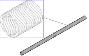
In the marine flatbed, nuclear power stations and oil fields, the marine risers (seen as Fig. 1) and heat exchangers [1, 2] are induced vibrations and collision, even caused failure with internal flow and external flow. This is a typical problem of bundles vibration in structure-interaction coupling. It related to multiple movable interfaces and multiple physical fields and which was difficult to calculate. Most of the results were studied the tube vibrations with internal flow and the vibration law was analyzed in longitudinally. M. Ragulskis [3] adopted harmonic balance method to study the non-Newtonian fluid flow in longitudinally vibrating tube. The tube vibrations induced by internal flow and the tube was a non-deformable rigid body. So far, the numerical methods for the tube vibrations with cross flow (external flow) are monolithic coupling algorithm and partitioned coupling algorithm [4-7]. In monolithic coupling algorithm, equations are solved simultaneously for fluid and structural domain. The advantage is the high accuracy [8, 9]. The disadvantage is that because the equations are integrated for fluid and structure and the solution efficiency is very low. Especially, it is not suitable for problems of large-scale and more complex domain. In partitioned coupling algorithm, equations are solved respectively. Within each time step or iteration, the information is transferred at the coupling interface. And the coupled solution is achieved. The advantage is that the solving range is wide and easy to conduct. The disadvantage is that the difference of grid density for fluid domain and structural domain at the coupling interface and which causes the grid do not match [10, 11]. Therefore, it need data transfer at the coupling interface. And it is the first to solve the problem in partitioned coupling algorithm. Comparing to the results of monolithic coupling algorithm, the error was small. The research outcome will make commutations of vibration and collision for bundles possible in a more complex fluid domain.

Fig. 1The tubes in engineering

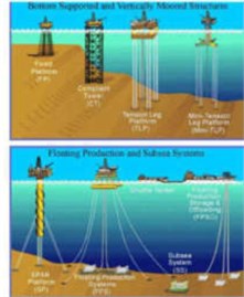
a) The marine risers in the ocean

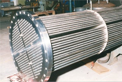
b) The heat exchanger tubes

2. The mechanics model of the coupling of elastic pipe and cross-flow in cylinder

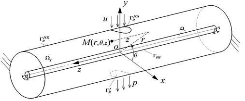
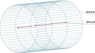
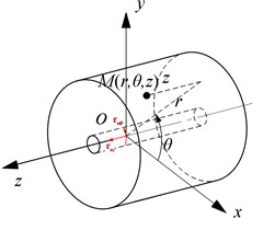
The fluid and elastic pipe was selected as research object in cylinder. The coupling mechanics model of the elastic pipe was set up. As shown in Fig. 2, the model was divided into two domains: the structural domain ${\Omega }_s$ and the fluid domain ${\mathrm{\Omega }}_f$. The assumptions were used as followed.

(1) The fluid medium is water. And it assumes the water is sticky and incompressible.

(2) The solid is assumed to be perfectly elastic body. And the elastic tube is prismatic. The cross section is always circular.

As shown in Fig. 1, the boundary of cylindrical entrance was velocity. And it was denoted by ${\mathrm{\Gamma }}_D^{f\left(1\right)}$. The boundary of outlet was pressure and it was denoted by ${\mathrm{\Gamma }}_N^f$. The boundary that the fluid was flowing along the inner cylinder’s wall surface was free slip and it was denoted by ${\mathrm{\Gamma }}_D^{f\left(2\right)}$. The interface between the fluid and solid interaction was fluid-structure coupling boundary and it denoted by ${\mathrm{\Gamma }}_{FSI}^{}$.

The boundary conditions for the cylinder fluid domain ${\mathrm{\Omega }}_f$ were:

where: ${\mathbf{n}}_r^f$, ${\dot{\mathbf{d}}}_r^f$, ${\mathbf{p}}_r$ were the vectors of normal unit, velocity, pressure, respectively. $u$ was inlet velocity and $p_0$ was outlet pressure. The superscripts of $f\text{,}$$s$ were represented fluid, solid respectively.

The structural domain ${\mathrm{\Omega }}_s$ was the elastic and the boundary was hinged on both ends.

Fig. 2The mechanics model of the elastic pipe and the cross-flow in cylinder

Supposed that the fluid and solid surface without sliding, the displacement and speed should meet the condition of coordination and the load should meet the condition of load balancing.

1) The condition of displacement coordination:

where: ${\mathbf{d}}^s$, ${\mathbf{d}}^f$ were the displacement vectors of solid and fluid respectively. ${\mathbf{n}}^s$, ${\mathbf{n}}^f$ were the unit displacement vectors of solid and fluid domain respectively. ${\mathbf{n}}^s={\mathbf{n}}_r^s+{\mathbf{n}}_{\theta }^s+{\mathbf{n}}_z^s\text{,}$${\mathbf{n}}^f={\mathbf{n}}_r^f+{\mathbf{n}}_{\theta }^f+{\mathbf{n}}_z^f$. ${\mathbf{n}}_r^s$, ${\mathbf{n}}_{\theta }^s$, ${\mathbf{n}}_z^s$ were unit vectors along the $r$, $\theta$, $z$ direction.

2) The condition of velocity coordination:

where: ${\dot{\mathbf{d}}}^f$, ${\dot{\mathbf{d}}}^f$ were the velocity vectors of solid and fluid respectively. ${\mathbf{n}}_{}^s$, ${\mathbf{n}}_{}^f$ were the same as the Eq. (2).

3) The condition of load balancing:

where: ${\mathbf{\sigma }}^s$, ${\mathbf{\sigma }}^f$ were the stress vectors of solid and fluid respectively.

3. The monolithic algorithm of the coupling of elastic pipe and the cross-flow in cylinder

3.1. The numerical model of the coupling of elastic tube and cross-flow with monolithic algorithm

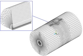
In monolithic algorithm, the fluid and were both divided by solid elements. The numerical model was shown in Fig. 3. The solid elements were adopted eight-node hexahedral element or six-node pentahedral element, as shown in Fig. 4.

Fig. 3The numerical model of transverse fluid and elastic tube with the method of universe

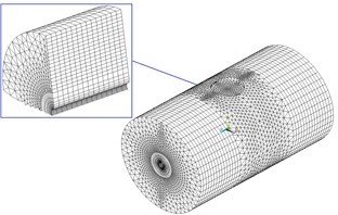
a) The finite element of cylindrical fluid

b) The finite element model of elastic tube

Fig. 4Solid element

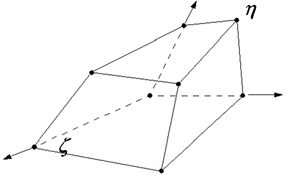
a) Hexahedral element

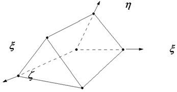
b) Pentahedral element

4. The partitioned algorithm of the coupling of elastic pipe and the cross-flow in cylinder

The monolithic algorithm is more accurate, the calculation is easier to implement. But the fluid and elastic tube are dispersed by solid element and the model is large which leads the low efficiency in monolithic algorithm. In particular, it is difficult to solve the coupling dynamics problem of tube bundle vibration and collision induced by cross-flow. Based on this, the paper presents a partitioned algorithm for calculating the vibration of elastic tube induced by cross-flow in a cylinder.

In monolithic algorithm, if we do not consider the coupling of cross-flow and elastic tube, the Eq. (7) can be simplified as:

The Eq. (8) is the control equation for fluid domain. The Eq. (9) is the dynamic equation for solid domain of the elastic tube. In partitioned algorithm, it is not necessary to solve the fluid-solid coupling Eq. (7). According to the set order, the Eqs. (8) and (9) are solved respectively. The information which calculated in fluid domain and solid domain are transferred to each other at fluid-solid interface (FSI) [14, 15]. Until the convergence of this time to meet the requirements, then the next moment of the calculation is carried. The final result will be obtained in repeated cycle.

4.1. The numerical model of the coupling of elastic tube and cross-flow with partitioned algorithm

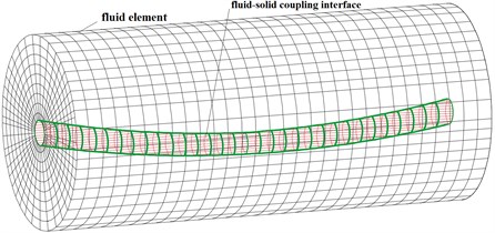
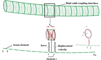
The numerical model of the coupling of elastic tube and cross-flow was seen as Fig. 5 with partitioned algorithm. Considering the slender beam characteristics of the elastic tube, the elastic tube was divided into several beam elements to improve the calculation scale and efficiency in partitioned algorithm. The coupling interface between fluid domain and solid domain of the elastic tube was shown in Fig. 6.

It can be seen from Fig. 5 and Fig. 6 that, due to the mismatch between solid element and elastic tube beam element at the coupling interface, the transfer information of displacement, velocity and force was deduced and partitioned algorithm for the coupling of cross-flow and elastic tube in the cylinder is achieved.

Fig. 5The numerical model of transverse fluid and elastic tube with partitioned method

a) The finite model element of fluid domain

b) The finite element model of elastic tube

Fig. 6The coupling interface

4.2. The information transfer between the elastic pipe and cross-flow in cylinder

The Fig. 7 showed the transitive relationship between the elastic pipe and cross-flow in cylinder at the coupling interface.

Fig. 7The transitive relationship between the elastic pipe and cross-flow

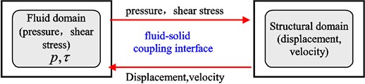
The red arrow from the fluid domain to structural domain was represented shear stress and pressure. Namely the fluid affected the elastic pipe by pressure, shear stress. The red arrow from the structural domain to fluid domain was represented displacement and velocity speed. Namely the elastic pipe transmitted displacement and velocity to fluid domain.

4.2.1. The information transmission of displacement and velocity at fluid-solid coupling interface

The information transmission of displacement and velocity was shown in Fig. 8. The beam element named $e$ was taken and its nodes were $i$ and $j$. The vectors of nodal displacement and velocity in local coordinate system were as followed:

10a

${\mathbf{d}}_e^s=[\begin{array}{llllllllllll}{u}_{ix}^s& u_{{}_{iy}}^s& u_{{}_{iz}}^s& {\theta }_{{}_{ix}}^s& {\theta }_{iy}^s& {\theta }_{iz}^s& u_{{}_{jx}}^s& u_{{}_{jy}}^s& u_{{}_{jz}}^s& {\theta }_{{}_{jx}}^s& {\theta }_{{}_{jy}}^s& {\theta }_{{}_{jz}}^s\end{array}{]}^{{\rm T}}$

10b

${\dot{\mathbf{d}}}_e^s=[\begin{array}{llllllllllll}{\dot{u}}_{ix}^s& {\dot{u}}_{{}_{iy}}^s& {\dot{u}}_{{}_{iz}}^s& {\dot{\theta }}_{{}_{ix}}^s& {\dot{\theta }}_{iy}^s& {\dot{\theta }}_{iz}^s& {\dot{u}}_{{}_{jx}}^s& {\dot{u}}_{{}_{jy}}^s& {\dot{u}}_{{}_{jz}}^s& {\dot{\theta }}_{{}_{jx}}^s& {\dot{\theta }}_{{}_{jy}}^s& {\dot{\theta }}_{{}_{jz}}^s\end{array}{]}^{{\rm T}}$

Fig. 8Force, displacement and velocity interpolation at coupling interface

a) The fluid element and fluid-solid coupling interface

b) The information transmission

The displacement and velocity of arbitrary axis position $x_m$ on the beam element was as followed by shape function $\mathbf{N}$:

11a

${\mathbf{d}}_{e,m}^s={\left[\begin{array}{llllll}{u}_{x,m}^s& u_{y,m}^s& u_{z,m}^s& {\theta }_{x,m}^s& {\theta }_{y,m}^s& {\theta }_{z,m}^s\end{array}\right]}^{{\rm T}}=N\left|{}_{x=x_m}\right.d_e^s$

11b

${\dot{\mathbf{d}}}_{e,m}^s={\left[\begin{array}{llllll}{\dot{d}}_{x,m}^s& {\dot{d}}_{y,m}^s& {\dot{d}}_{z,m}^s& {\dot{\theta }}_{x,m}^s& {\dot{\theta }}_{y,m}^s& {\dot{\theta }}_{z,m}^s\end{array}\right]}^{{\rm T}}=N\left|{}_{x=x_m}\right.{\dot{d}}_e^s$

According to the assumption that the cross section was always circular, the displacement components of the node $k$ at axis position $x_m$ was as followed:

12

$\left\{\begin{array}{l}{u}_{x,m}^f=u_{x,m}^s+r\mathrm{s}\mathrm{i}\mathrm{n}{\theta }_{y,m}^s\mathrm{s}\mathrm{i}\mathrm{n}{\theta }_k-r\mathrm{s}\mathrm{i}\mathrm{n}{\theta }_{z,m}^s\mathrm{c}\mathrm{o}\mathrm{s}{\theta }_k,\\ u_{y,m}^f=u_{y,m}^s+r\mathrm{c}\mathrm{o}\mathrm{s}\left({\theta }_{x,m}^s+{\theta }_k\right)-r\mathrm{c}\mathrm{o}\mathrm{s}{\theta }_k,\\ u_{z,m}^f=u_{z,m}^s+r\mathrm{s}\mathrm{i}\mathrm{n}\left({\theta }_{x,m}^s+{\theta }_k\right)-r\mathrm{s}\mathrm{i}\mathrm{n}{\theta }_k,\end{array}\right.$

where, $r$ was outer radius of the elastic pipe. $x_m$ was distance from the node $i$. ${\theta }_k$ was circumferential angle of node $k$, which was shown in Fig. 8.

The displacement vector ${\mathbf{d}}_{e,m}^f$ can be expressed as:

13

${\mathbf{d}}_{e,m}^f={\left[\begin{array}{lll}{u}_{x,m}^f& u_{y,m}^f& u_{z,m}^f\end{array}\right]}^{{\rm T}}={\mathbf{H}}_{FSI}^e{\mathbf{d}}_{e,m}^s={\mathbf{H}}_{FSI}^{e}N\left|{}_{x=x_m}\right.{\mathbf{d}}_e^s$

where, ${\mathbf{H}}_{FSI}^e$ was the displacement transformation matrix from structural domain to fluid domain.

Assigned ${\mathbf{H}}_{{\mathrm{\Gamma }}_{FSI}}^e={\mathbf{H}}_{FSI}^{e}N\left|{}_{x=x_m}\right.$, then the displacement, velocity vector of the fluid units on the fluid-solid coupling interface can be expressed as:

14a

${\mathbf{d}}_{e,m}^f={\mathbf{H}}_{{\mathrm{\Gamma }}_{FSI}}^e{\mathbf{d}}_e^s$

14b

${\dot{\mathbf{d}}}_{e,m}^f={\mathbf{H}}_{{\mathrm{\Gamma }}_{FSI}}^e{\dot{\mathbf{d}}}_e^s$

Thence, the displacement, velocity vector of the fluid at time $t$ can be expressed as:

15a

${\mathbf{d}}_{e,m}^f\left(t\right)={\mathbf{H}}_{{\mathrm{\Gamma }}_{FSI}}^e\left(t\right){\mathbf{d}}_e^s\left(t\right)$

15b

${\dot{\mathbf{d}}}_{e,m}^f\left(t\right)={\mathbf{H}}_{{\mathrm{\Gamma }}_{FSI}}^e\left(t\right){\dot{\mathbf{d}}}_e^s\left(t\right)$

When the elastic pipe was deformed, according to the Eq. 15(a) and 15(b), the displacement and velocity would be re-applied on the boundary wall in fluid domain. Therefore, the coordination of displacement and velocity was achieved at the fluid-solid coupling interface.

4.2.2. The information transmission of load at the fluid-solid coupling interface

As shown in Fig. 9, the interface loads were obtained at the outer surface of the elastic pipe in fluid domain. And the loads were decomposed into normal pressure $p$, tangential shear stress ${\tau }_{r\varphi }$ and axial shear stress ${\tau }_{rx}$. First, loads were integrated along the surface and simplified at the corresponding axis. Then according to the principle of virtual work, loads were equivalent to the values of nodes $i$, $j$ of beam element.

Fig. 9The interface loads at the outer surface of the elastic pipe in fluid domain

a) Space

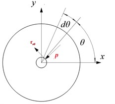
b) Plane

In the beam element at $x=x_m$, the length of element was $L_{x_m}$.The forces and torques was simplified was as followed:

16

$\left\{\begin{array}{l}{q}_{F_x}^m={\int }_0^{L_{x_m}}{\int }_0^{2\pi }\left({\tau }_{r\theta }\mathrm{s}\mathrm{i}\mathrm{n}\theta +P\mathrm{c}\mathrm{o}\mathrm{s}\theta \right)d\theta dz,\\ q_{F_y}^m={\int }_0^{L_{x_m}}{\int }_0^{2\pi }\left({\tau }_{r\theta }\mathrm{c}\mathrm{o}\mathrm{s}\theta +P\mathrm{s}\mathrm{i}\mathrm{n}\theta \right)d\theta dz,\\ q_{F_z}^m={\int }_0^{L_{x_m}}{\int }_0^{2\pi }{\tau }_{rz}d\theta dz,\\ q_{m_x}^m=r{\int }_0^{L_{x_m}}{\int }_0^{2\pi }{\tau }_{r\theta }\mathrm{s}\mathrm{i}\mathrm{n}\theta d\theta dz,\\ q_{m_y}^m=r{\int }_0^{L_{x_m}}{\int }_0^{2\pi }{\tau }_{r\theta }\mathrm{c}\mathrm{o}\mathrm{s}\theta d\theta dz,\\ q_{m_z}^m=r{\int }_0^{L_{x_m}}{\int }_0^{2\pi }{\tau }_{rz}d\theta dz.\end{array}\right.$

The Eq. (16) was represented by a vector:

17

${\mathbf{q}}_m^f=[\begin{array}{llllll}{q}_{F_x}^m& q_{F_y}^m& q_{F_z}^m& q_{m_x}^m& q_{m_y}^m& q_{m_z}^m\end{array}{]}^T$

According to the principle of virtual work, the above-mentioned axial loads were further equivalent to values of the node on beam elements:

18

${\mathbf{F}}_e^f=\sum _{m=1}^{n_{fo}^x}{\mathbf{F}}_f^i=\sum _{m=1}^{n_{fo}^x}{\mathbf{T}}^T{\int }_0^{L_{x_m}}{\mathbf{N}}^T{\mathbf{q}}_m^{f}dx,$

where, $\mathbf{T}$ was the converted matrix of coordinates.

All nodal loads which were equivalent to the beam element were assembled. Then, the equivalent nodal loads ${\mathbf{F}}_f\left(t\right)$ were obtained from the fluid domain to the elastic pipe. Thus, it met the conditions of load balancing at the coupling interface.

Substituted ${\mathbf{F}}_f\left(t\right)$ into the dynamic Eq. (9) of the elastic pipe, the dynamic equations of the elastic pipe was obtained as followed when considering the effect of fluid:

19

$\mathbf{M}{\ddot{\mathbf{d}}}_{}^s+\mathbf{C}{\dot{\mathbf{d}}}_{}^s+\mathbf{K}{\mathbf{d}}_{}^s={\mathbf{F}}_s+{\mathbf{F}}_f$

where, the ${\mathbf{F}}_f$ was the vector of fluid force at the coupling interface.

4.4. The frame diagram of partitioned algorithm for elastic pipe and cross-flow in cylinder

The Fig. 10 was the total frame diagram of partitioned algorithm. $t_{end}$ was the total computational time. The iterative process was as followed.

(1) The models of fluid domain and structural domain were established. Give inlet velocity u and outlet pressure $P$. Give the initial displacement and initial velocity at the coupling interface.

(2) Solve the fluid domain ${\mathrm{\Omega }}_f$ and get the coupling interface load $F_{\mathrm{\Gamma }f}^{jk}\left(t\right)$;

(3) According to the Eq. (18), get the coupling interface loads $\mathbf{F}\left(t\right)$ of structural domain;

(4) Solve structural domain ${\mathrm{\Omega }}_s$, get displacement and velocity at coupled interface in structural domain.

(5) According to the Eq. (15), get the displacement ${\mathbf{d}}_{\mathrm{\Gamma }s}^{jk}\left(t\right)$ and velocity ${\mathbf{u}}_{\mathrm{\Gamma }s}^{jk}\left(t\right)$ at coupled interface in fluid domain.

(6) According to the convergence Eq. (20), if the values of displacement, velocity and load do not meet the convergence criteria, return the coupled iteration from the Eq. (3) to Eq. (6).

(7) If the values of displacement, velocity and load meet the convergence Eq. (20) at the same time, Order $t=t+\mathrm{\Delta }t$, follow the previous coupling step Eq. (2) to (6). Otherwise, end of the iteration.

The coupling iteration loop at the current time step was seen as the Fig. 11.

In partitioned algorithm of the elastic pipe and the cross-flow in cylinder, the data of displacement, velocity and load was transferred with the time. The process of time-step cycle was seen in Fig. 12.

Fig. 10The total frame diagram of partitioned algorithm

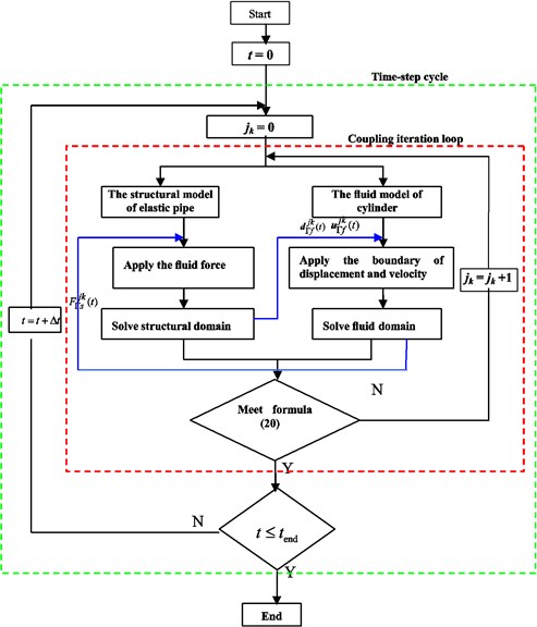
Fig. 11The calculation process at the current time step

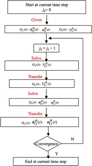
Fig. 12The process of time-step cycle

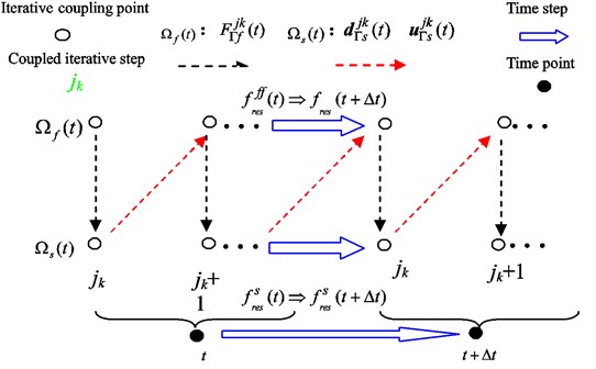
Seen from the Fig. 12, the results files $f_{{}_{res}}^f\left(t\right)$, $f_{{}_{res}}^s\left(t\right)$ of fluid domain and structural domain were used as initial values at time $t$. Then solving the fluid domain and structural domain at time $t+\mathrm{\Delta }t$, the results files $f_{{}_{res}}^f(t+\mathrm{\Delta }t)$, $f_{{}_{res}}^s(t+\mathrm{\Delta }t)$ were obtained. And the $F_{\mathrm{\Gamma }f}^{}(t+\mathrm{\Delta }t)$ in fluid domain, the ${\mathbf{d}}_{\mathrm{\Gamma }f}^{}(t+\mathrm{\Delta }t)$ and ${\mathbf{u}}_{\mathrm{\Gamma }f}^{}(t+\mathrm{\Delta }t)$ in structural domain were taken at the same time. Thus, these physical quantities would be initial values at time $t+\mathrm{\Delta }t$.

5. Examples and verification

5.1. Cases and calculation parameters

The calculation parameters of the elastic pipe and fluid were listed in Table.

Table 1The calculation parameters of the elastic pipe and fluid

Length (m)	0.5
Outer diameter (m)	0.02
Inner diameter (m)	0.016
Elastic modulus (GPa)	3.5
Poison’s ratio	0.3
The density of elastic pipe (kg/m3)	2250
The density of fluid(kg/m3)	1000
Dynamic viscosity (mPa.s)	1
Inlet velocity (m/s)	2.236
outlet pressure (MPa)	0
Natural frequency of elastic pipe (Hz)	23.91
Calculation time step (s)	0.001

Fig. 13The path I and cross section II in the model

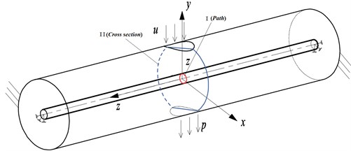
As shown in Fig. 1, the elastic was placed at the center in cylinder. The elastic pipe in the cylinder fluid was calculated by the monolithic and partitioned algorithm respectively. Then the vortex-induced vibration of the elastic was obtained in solid domain. And the distribution of the pressure and velocity were also obtained in fluid domain. The corresponding results were compared by the two calculation methods. The path I and cross section II of the elastic pipe was shown in Fig. 13. The contrast results of the elastic pipe in solid domain were shown in Fig. 14 and Fig. 15 and the values were listed in Table 2 along the path I. The contrast results in fluid domain were shown in Fig. 16 and Fig. 17 and the values were listed in Table 3 at cross Section 2.

5.1.1. The contrast results of elastic pipe in solid domain.

Seen from Fig. 14(a), (b) and (c), the curves of the acceleration, velocity, displacement were identical by the methods of monolithic and partitioned for the elastic pipe. From Table 2, the maximum error of the acceleration amplitude was 5.33 % at time 0.0s – 0.3s. And the maximum error of the velocity amplitude was 4.90 % for the elastic pipe. And the maximum error of the displacement amplitude was 4.20 %. All error is less than 5 %. Hence, it presented the correctness of the partitioned algorithm for the coupling of the elastic pipe and the cross-flow in cylinder.

Fig. 14The contrast curves of acceleration, velocity, displacement for the elastic pipe

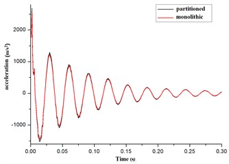
a) Acceleration

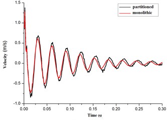
b) Velocity

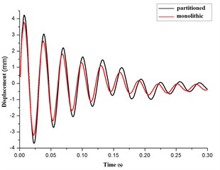
c) Displacement

Table 2The amplitude list of the acceleration, velocity, displacement

Time period (s)			0-0.03	0.03-0.06	0.06-0.09	0.09-0.12	0.12-0.15
Acceleration	Amplitude (m/s2)	Monolithic	4006	2267	1615	1101	771
		Partitioned	4015	2272	1632	1118	786
	Error (%)		0.22	0.22	1.05	1.54	1.94
Velocity	Amplitude (mm/s)	Monolithic	2011	1130	790	555	395
		Partitioned	2079	1152	798	561	401
	Error (%)		3.38	1.95	1.01	1.08	1.52
Displacement	Amplitude (mm)	Monolithic	7.32	5.59	4.03	2.99	2.09
		Partitioned	7.90	5.79	4.23	3.05	2.19
	Error (%)		7.92	3.58	4.96	2.01	4.78
Time period (s)			0.15-0.18	0.18-0.21	0.21-0.24	0.24-0.27	0.27-0.30
Acceleration	Amplitude (m/s2)	Monolithic	514	348	251	197	150
		Partitioned	521	352	258	203	158
	Error (%)		1.36	1.15	2.79	3.05	5.33
Velocity	Amplitude (mm)	Monolithic	235	186	132	102	82
		Partitioned	239	189	136	107	85
	Error (%)		1.70	1.61	3.03	4.90	3.66
Displacement	Amplitude (m/s2)	Monolithic	1.86	1.19	0.70	0.60	0.39
		Partitioned	1.92	1.24	0.72	0.62	0.42
	Error (%)		3.23	4.20	2.86	3.33	7.69

5.1.2. The contrast results of pressure and velocity distribution in fluid domain

The distribution of pressure and velocity was shown as Fig. 15 along path I in fluid domain at $t=$ 0.281 s.

Seen from Fig. 15, the distribution of pressure and velocity was identity by the algorithm of monolithic and partitioned coupling along path I. Of note, in 48°-132°, namely in the position of upstream face, the fluid pressure was positive, greater than atmospheric pressure and the maximum value was at the position of 90°. In 132°-210°, 330°-360°, 0°-48°, namely in the position of side face, the fluid pressures were relatively negative, less than atmospheric pressure and the maximum negative value was occurred in 174° and 6° position. In 220°-320°, namely in the position of lee face, the fluid pressures were relatively positive, greater than atmospheric pressure. But the values were smaller than values of upstream face.

Seen from the Table 3, the errors of pressure calculated by the two methods were –0.17 %, 0.04 %-0.87 %, 0.15 % respectively, in the location of 6°, 90°, 174°, 27° along path I. And the errors of velocity were –0.27 %, 1.71 %, –0.27 %, –1.35 % respectively. Therefore, the values of pressure and velocity obtained by the two methods were equivalent in the fluid domain.

Fig. 15The pressure and velocity distribution along path I

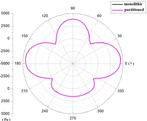
a) Pressure

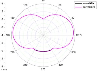
b) Velocity

Table 3The list of the pressure and velocity along path I

Positions (°)	Pressure			Velocity
	Monolithic (Pa)	Partitioned (Pa)	Error (%)	Monolithic (m/s)	Partitioned (m/s)	Error (%)
6	–4589.70	–4581.91	–0.17	–3.73	–3.72	–0.27
90	3896.77	3898.17	0.04	–0.115	–0.117	1.71
174	–4590.43	–4550.63	–0.87	–3.68	–3.67	–0.27
270	1552.97	1555.29	0.15	0.075	0.074	–1.35

Fig. 16The pressure and velocity contours at cross section II by monolithic algorithm

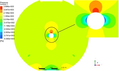
a) Pressure

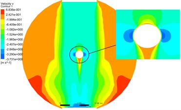
b) Velocity

Fig. 17The pressure and velocity contours at cross Section 2 by partitioned algorithm

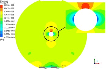
a) Pressure

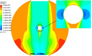
b) Velocity

The Fig. 16 and Fig. 17 were pressure and velocity contours at cross Section 2 by monolithic and partitioned algorithm. From the contours, the distribution of pressure and velocity at cross Section 2 were basically the same.

6. Conclusions

1) The coupling mechanics model was established for the elastic pipe and the cross-flow in cylinder. The boundary conditions of the inlet flow rate, outlet pressure and wall were considered in the model. And it also met the conditions of displacement, velocity and load balancing at fluid-structure coupling interface.

2) In monolithic algorithm, the model of fluid and elastic tube is both dispersed by solid elements. The dynamic coupling finite element equation was applied to solve the dynamic characteristics of elastic pipe in solid domain and the velocity and pressure in fluid domain. Although the monolithic algorithm is easy and accurate, the model is very lager in general and it may lead a low efficiency. In particular, it is difficult to solve the coupling dynamics problem of multiple bundles vibration and collision induced by cross-flow in a more complex fluid domain. Based on this, the partitioned algorithm was established for elastic pipe and cross-flow in cylinder. In partitioned algorithm, the elastic pipe was separated into several beam elements. The cross-flow was still separated into solid elements. At the fluid-structure coupling interface, the formulas of displacement, velocity and load was derived and the corresponding convergence criterion was also derived. The iterative block diagram of partitioned coupling algorithm was designed.

3) According the above two methods, the example was calculated by the algorithm of monolithic and partitioned. The results proved that the curves of acceleration, velocity, displacement for elastic pipe were consistent by two algorithms in solid domain. And pressure and velocity distribution were also consistent by two algorithms at cross section II in fluid domain. It proved the correctness of the partitioned coupling algorithm which was established in this article.

4) The method will provide an effective computational method for vibrations and collision of multiple bundles in a more complex fluid domain. And it will have important theoretical significance in engineering.