An automatic feature extraction method and its application in fault diagnosis

Wang, Jinrui; Li, Shunming; Jiang, Xingxing; Cheng, Chun

doi:10.21595/jve.2017.17906

Journal of Vibroengineering

Browse Journal

Submit article

Published: 30 June 2017

Check for updates

An automatic feature extraction method and its application in fault diagnosis

Jinrui Wang¹

Shunming Li²

Xingxing Jiang³

Chun Cheng⁴

^{1, 2, 3, 4}College of Energy and Power Engineering, Nanjing University of Aeronautics and Astronautics, Nanjing 210016, P. R. China

³School of Urban Rail Transportation, Soochow University, Suzhou 215137, P. R. China

Corresponding Author:

Shunming Li

Cite the article Download PDF

Downloads 1620

WoS Core Citations 5

CrossRef Citations 9

Abstract

The main challenge of fault diagnosis is to extract excellent fault feature, but these methods usually depend on the manpower and prior knowledge. It is desirable to automatically extract useful feature from input data in an unsupervised way. Hence, an automatic feature extraction method is presented in this paper. The proposed method first captures fault feature from the raw vibration signal by sparse filtering. Considering that the learned feature is high-dimensional data which cannot achieve visualization, $t$ -distributed stochastic neighbor embedding ( $t$ -SNE) is further selected as the dimensionality reduction tool to map the learned feature into a three-dimensional feature vector. Consequently, the effectiveness of the proposed method is verified using gearbox and bearing experimental datas. The classification results show that the hybrid method of sparse filtering and $t$ -SNE can well extract discriminative information from the raw vibration signal and can clearly distinguish different fault types. Through comparison analysis, it is also validated that the proposed method is superior to the other methods.

1. Introduction

As the most essential system in rotating machinery, gear and bearing play a major role to keep the entire machine operating normally. Serious faults of gear and bearing may lead to catastrophic consequences and cause enormous economic losses. So, condition monitoring and fault diagnosis have attracted broad attention in reducing undesirable casualties and minimizing production loss [1].

The feature extracted from vibration signal is commonly used to detect faults in machines [2]. And the more meaningful feature can enhance the identification accuracy. However, complex structures and noises in the observed signal make it difficult to extract the effective feature. For this reason, Different kinds of signal processing methods have been performed such as time-domain analysis [3], frequency transform [4], time-frequency analysis [5, 6] and envelope demodulation [7]. Among the conventional methods, researchers have spent a large amount of time on feature extraction and selection which are complicated and longstanding tasks. With the research of machine learning, neural network [8, 9] has attracted more and more attention. It can automatically learn high-dimensional feature from the signal by the hidden layers, but it still requires lots of label data.

As a viable alternative to manually design feature representations, unsupervised feature learning has been successfully implemented to extract good characteristics in many image [10], video [11] and audio [12] tasks. However, many current unsupervised feature learning algorithms are challenging to implement because they need to turn the various hyperparameters. If the hyperparameters are set improperly, it will produce a great impact on the diagnosis accuracy [13]. These algorithms include sparse RBMs [14], sparse autoencoders [15], sparse coding [16], independent component analysis (ICA) [17] and others. A comparison of the tunable hyperparameters in these algorithms are shown in Table 1. For instance, Sparse RBMs has up to half a dozen hyperparameters which makes it difficult to tune and monitor convergence. ICA has just one tunable hyperparameter, but it scales poorly to large inputs or large sets of features [18]. Ngiam et al. [19] proposed an unsupervised feature learning network named sparse filtering. It only focuses on optimizing the sparsity of the learned representations and ignores the problem of learning the data distribution. It also scales excellently with the dimension of the input. Only the number of features needs to set, so it is extremely simple to tune and easy to implement by a few lines of MATLAB code. Meanwhile in Ref. [19], the author adopted it on image recognition and phone classification, which generated the state-of-the-art performance.

Table 1Tunable hyperparameters in various algorithm

Algorithm	Tunable hyperparameters
Sparse filtering	Features
ICA	Features
Sparse coding	Features, sparse penalty, mini-batch size
Sparse autoencoders	Features, weight decay, target activation, sparse penalty
Sparse RBMs	Features, weight decay, target activation, sparse penalty, learning rate, momentum

Because of its simplicity and performance, sparse filtering is proposed to solve fault diagnosis of rotating machines in this paper. However, the dimension of the learned feature is too high so that visualization is difficult. So, it is necessary to select a suitable dimensionality reduction tool to embed the learned feature into a low-dimensional space. Maaten et al. [20] introduced an nonlinear dimensionality reduction technique called $t$ -distributed stochastic neighbor embedding ( $t$ -SNE), which is more effective in creating a single map at different scales than other techniques. Then the reduced features of different fault types can achieve visualization in a scatter plot.

This paper is organized as follows. Section 2 briefly introduces the algorithms of sparse filtering and $t$ -SNE. Section 3 is dedicated to detail the content of the proposed method. In Sections 4, the diagnosis cases of gearbox and bearing datasets are adopted to validate the effectiveness of the proposed method. Furthermore, the superiority of the proposed method is exhibited by comparing with other methods. Finally, the conclusion is drawn in Section 5.

2. Theoretical background

2.1. Sparse filtering

Sparse filtering is a simple unsupervised two-layer network which aims to optimize the sparsity of the learned features but not attempts to model the data distribution [19]. The method learns the excellent features in an unsupervised way which possesses three principles:

(1) Population sparsity: each sample should be sparsity, which means each sample is represented by just a few activated elements.

(2) Lifetime sparsity: each feature should be sparsity, which means each feature allows to be activated only for a small number of samples.

(3) High dispersal: each feature should have similar statistical properties.

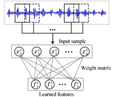
The architecture of sparse filtering is shown in Fig. 1. The collected raw vibration signal is directly used as the input data. Firstly, the vibration signal is separated into $M$ samples to compose a training set ${x^{i}}_{i = 1}^{M}$ , where $x^{i} \in R^{N \times 1}$ is a training sample contains $N$ data points. Then, the training set is used to train the sparse filtering model so as to obtain a weight matrix $W \in R^{N \times L}$ . Finally, each sample is mapped into a feature vector $f^{i} \in R^{L \times 1}$ by the weight matrix $W$ . For sparse filtering, an activation function is needed for calculating the nonlinear features. In our experiment, the soft-absolute function is adopted as the activation function and the features of each sample can be calculated as follows:

1

f_{j}^{i} = \sqrt{ε + {(W_{j}^{T} x^{i})}^{2}} \approx |W_{j}^{T} x^{i}|

where $f_{j}^{i}$ is the $j$ th feature value corresponding to rows in the $i$ th column, $ε =$ 10^-8.

The feature matrix is comprised by the features $f_{j}^{i}$ . Firstly, each row is normalized to be equally active by its $l 2$ -norm:

2

{\tilde{f}}_{j} = \frac{f_{j}}{| | f_{j} | |_{2}} .

Then, each column (or each sample) is normalized by its $l 2$ -norm. As a result, each feature is constrained to lie on the unit $l 2$ -ball:

3

{\hat{f}}^{i} = \frac{{\tilde{f}}^{i}}{| | {\tilde{f}}^{i} | |_{2}} .

At last, the normalized features are optimized for sparseness using the $l 1$ penalty. For the training set ${x^{i}}_{i = 1}^{M}$ , the sparse filtering objective is shown as follows:

4

\underset{W}{m i n i m i z e} \sum_{i = 1}^{M} | | {\hat{f}}^{i} | |_{1} .

Fig. 1Architecture of sparse filtering

2.2. T-SNE

As a nonlinear dimensionality reduction technique, $t$ -SNE is extremely suited for embedding the high-dimensional dataset into an $s$ -dimensional vector (typical values for $s$ are 2 or 3) [21]. So, each object can be represented by a point in the scatter plot. To this end, $t$ -SNE determines the joint probabilities $p_{i j}$ that measure the pairwise similarity between features $f_{i}$ and $f_{j}$ by symmetrizing two conditional probabilities as follows:

5

p_{j | i} = \frac{e x p (- {‖f_{i} - f_{j}‖}^{2} / 2 σ_{i}^{2})}{\sum_{k \neq i} e x p (- {‖f_{i} - f_{k}‖}^{2} / 2 σ_{i}^{2})},

6

p_{i j} = \frac{p_{i | j} + p_{j | i}}{2 N},

where ${σ_{i}}^{2}$ is the variance of the Gaussian, which is centered on feature $f_{i}$ and is determined by the way that the perplexity of the conditional distribution equals to a predefined perplexity. As a result, $σ_{i}$ tends to be smaller in the data space with a higher data density than a lower data density. So, for each input object, the optimal value of $σ_{i}$ can be found using a simple binary search.

In the low-dimensional space, the similarities between two features $y_{i}$ and $y_{j}$ (i.e., the mapped features of $f_{i}$ and $f_{j}$ ) are measured using a normalized heavy-tailed kernel. Specifically, the joint probabilities $q_{i j}$ between $y_{i}$ and $y_{j}$ is computed as a normalized Student-t distribution:

7

q_{i j} = \frac{{(1 + {‖y_{i} - y_{j}‖}^{2})}^{- 1}}{\sum_{k \neq l} {(1 + {‖y_{k} - y_{l}‖}^{2})}^{- 1}} .

The heavy tails of the normalized Student-t distribution can make the input objects $f_{i}$ and $f_{j}$ to be modeled far apart by $y_{i}$ and $y_{j}$ . And it creates more space to accurately model the small pairwise distance. The locations of the embedding points $y_{k}$ are computed by minimizing the KL divergence between the joint distributions $q_{i j}$ and $p_{i j}$ :

8

K L (P | | Q) = \sum_{i \neq j} p_{i j} l o g (\frac{p_{i j}}{q_{i j}}),

where $P$ and $Q$ are the matrix formation of $p_{i j}$ and $q_{i j}$ . Then $f_{k}$ and $y_{k}$ are becoming more and more similar with each other. That is to say, $y_{k}$ could represent the characteristics of $f_{k}$ .

3. Proposed framework

This section details how to automatically extract features from mechanical signal. The procedure of our method is displayed in Fig. 2 and it can be described as following:

Fig. 2Flowchart of the proposed method

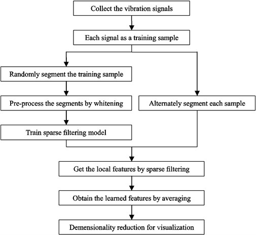
(1) Collect signals. The vibration signals are collected under different health conditions and are directly adopted as the training samples. We collect $Z$ segments from each sample to compose the training set ${\{s^{j}\}}_{j = 1}^{Z}$ by an overlapped manner, where $s^{j} \in R^{N_{i n} \times 1}$ is the $j$ th segment containing $N_{i n}$ data points.

(2) Whitening. The training set ${\{s^{j}\}}_{j = 1}^{Z}$ is written as a matrix formation $S \in R^{N_{i n} \times Z}$ and pre-processed by whitening. In this way, the segments can become less correlated with each other and the convergence rate can get faster [22]. By computing:

9

c o v (S^{T}) = E U E^{T},

where $c o v (S^{T})$ is the covariance matrix, $E$ denotes the orthogonal matrix of eigenvectors, and $U$ is the diagonal matrix of the eigenvalues. Then the whitened training set $S_{w}$ can be obtained as follows:

10

S_{w} = E U^{- 1 / 2} E^{T} S .

(3) Train sparse filtering. $S_{w}$ is employed to train the sparse filtering model, and then the weight matrix $W$ is obtained by minimizing Eq. (4).

(4) Calculate the local features. The training sample $x^{i}$ is alternately divided into $K$ segments, where $K = N / N_{i n}$ And these segments constitute a set ${\{{x_{k}}^{i}\}}_{k = 1}^{K}$ , where $x_{k}^{i} \in R^{N_{i n} \times 1}$ . Then the local features $f_{k}^{i} \in R^{1 \times N_{o u t}}$ can be calculated from each training sample $x_{k}^{i}$ by the weight matrix $W$ .

(5) Obtain the learned features. The local features $f_{k}^{i}$ are combined into a feature vector $f^{i}$ by the method of averaging, and $f^{i}$ is the learned feature:

11

f_{}^{i} = {(\frac{1}{K} \sum_{k = 1}^{K} f_{k}^{i})}^{T} .

(6) Dimensionality reduction. Since the obtained feature $f^{i}$ is still high-dimensional data, $t$ -SNE is adopted to reduce its dimension for visualization.

4. Fault diagnosis using the proposed method

In this section, a gearbox and a bearing experimental datasets are employed to validate the effectiveness of our method. In order to further illustrate the superiority of our method, several commonly used dimensionality reduction tools are adopted to combine with sparse filtering respectively for comparison analysis.

4.1. Case 1. Gearbox experiment verification

4.1.1. Data description

A four-speed motorcycle gearbox [23] is used to collect vibration signals as shown in Fig. 3. Besides the gearbox, there are an electrical motor, a tachometer, a tri-axial accelerometer, a data acquisition system, a load mechanism and four shock absorbers. There are four kinds of gearbox defects under a certain load: normal condition (NC), slight-worn (SW), medium-worn (MW) and broken-tooth (BT), as shown in Fig. 3. The sampling frequency was 16384 Hz. We collect 50 samples from the raw vibration singal of NC and 100 samples from the raw vibration signal of SW, MW and BT, where each sample contains 1200 data points.

4.1.2. Diagnosis results

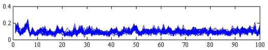
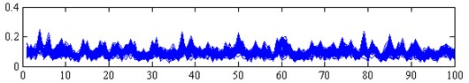
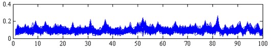
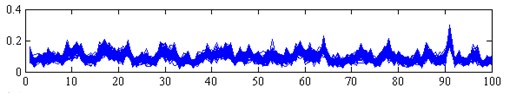
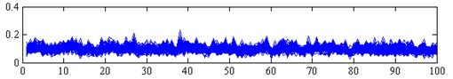
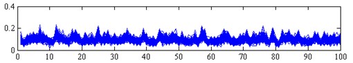
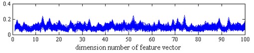
In this subsection, we will process the dataset by the proposed method. Firstly, we randomly select 10 % samples from each health condition to train the sparse filtering model. And then we randomly select 50 segments from each sample by using an overlapped manner, where each segment contains 100 data points. These segments are employed to constitute the training set ${\{s^{j}\}}_{j = 1}^{50}$ , where $s^{j} \in R^{100 \times 1}$ is the $j$ th segment containing 100 data points. Subsequently, we use these samples to train the sparse filtering model. There are two tunable feature parameters, i.e., the input and output dimension ( $N_{i n}$ and $N_{o u t}$ ). Ref. [24] investigated the selection of these two parameters. It randomly selected 10 % of samples to train and the rest to test. The diagnosis results showed that the larger $N_{i n}$ is, the more time spends. Considering that the testing accuracy of $N_{i n} =$ 100 is the highest and the spent time is low, so $N_{i n}$ is identified as 100. And the selection of $N_{o u t}$ is tradeoff between the diagnosis accuracy and the spent time. Since the increasing of the accuracy is not obvious after $N_{o u t} =$ 100, so $N_{o u t}$ is also identified as 100. After the sparse filtering model is trained and the weight matrix $W$ is obtained, we use the rest samples to calculate the learned features by the weight matrix $W$ . Each sample is alternately divided into 12 segments, where each segment contains 100 data points. As a result, a 100-dimensional feature vector is obtained for each $s^{j}$ as show in Eq. (11). In Fig. 4, it exhibits all the learned feature vectors of each health condition. It can be observed that the dimension of the learned feature is too high so that visualization is difficult. Finally, $t$ -SNE is adopted to embed the learned feature into a three-dimensional feature vector for visualization.

Fig. 3a) Experimental set up; b) worn teeth; c) worn model; d) broken teeth; e) schematic of the gearbox; and f) accelerometer location

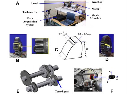
Fig. 4Learned feature vectors of gearbox

a) NC

b) SW

c) MW

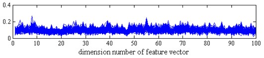
d) BT

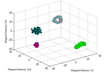
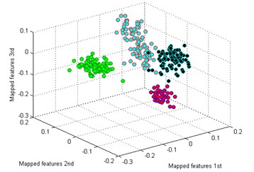
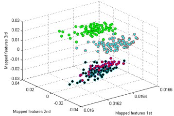
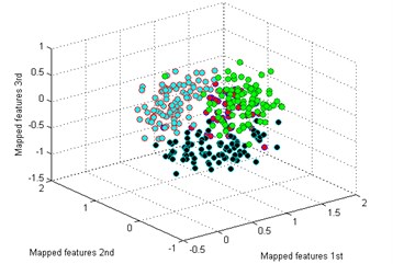
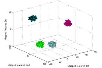
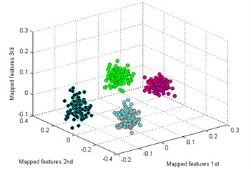
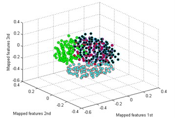
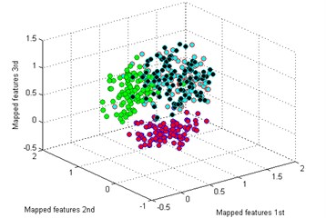
The classification result by our method is shown in Fig. 5(a). It is seen that the mapped features of the different types are separated excellently and the features of the same type are gathered together, and the distance between each type is large enough for distinguishing different health conditions. In addition, two similar models of worn gear are separated clearly. To testify the superiority of our method, five common dimensionality reduction tools combined with sparse filtering are adopted to process the gearbox dataset respectively. The five tools are: principal component analysis (PCA) [25], locality preserving projection (LPP) [26], Sammon mapping (SM) [27], linear discriminant analysis (LDA) [28], and stochastic proximity embedding (SPE) [29]. The classification results by the five methods are shown in Fig. 5(b)-(f).

Fig. 5Visualize features of gearbox

a) T-SNE

b) PCA

c) SM

d) LPP

e) LDA

f) SPE

By comparing the results of the six methods, it is easy to see that the classification by $t$ -SNE is the best. The mapped features by PCA are shown in Fig. 5(b), and its classification result is better than the rest methods. But there is still a big gap with the proposed method. For instance, the mapped features of MW are not well clustered and several of them are mixed with BT. In Fig. 5(c) which exhibits the mapped features by SM. In fact, these features are separated from another view to see. But the distance between each type is too small to distinguish. As we noticed in Fig. 5(d), the mapped features of NC and BT are almost mixed together which show a bad performance by LPP. In Fig. 5(e), it can be observed that the mapped features by LDA are not separated out at all, which shows it cannot be used for classification. And in Fig. 5(f) which displays the mapped features by SPE is also not performed very well. Through the above comparison analysis, it is indicated that our method is the best choice for discriminating different fault types of the gearbox dataset.

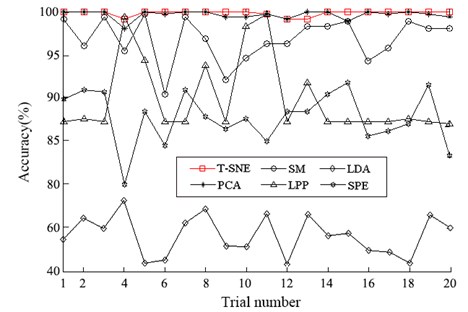
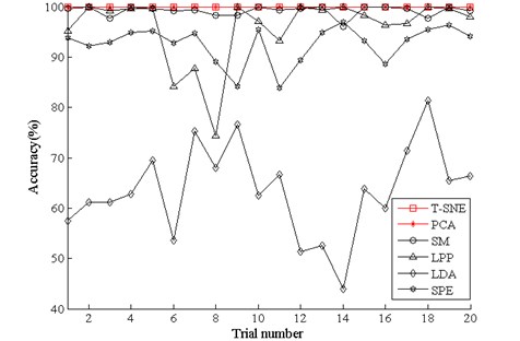
Furthermore, to illustrate the advantage of the proposed method. softmax regression [30] is adopted as the classifier to test the accuracies of the mapped features by the six methods. We randomly select 10 % samples from each health condition to train the softmax regression model and the rest to test. The weight decay term $λ$ of softmax regression is 1E-5. To reduce the effects of randomness, 20 trials are carried out for the experiment. The diagnosis results are depicted in Fig. 6. It shows that the diagnosis accuracies of $t$ -SNE and PCA vary a little and the other methods vary greatly. As we can notice that the performance of $t$ -SNE is a little better than PCA. Then the test accuracies are averaged by 20 trials and the results are displayed in Table 2. It can be seen that the average testing accuracy of the proposed method is 99.87 %, which is the best of all. And the accuracies of all the methods are the same as the performances of the visualize features in Fig. 5.

To verify the effectiveness of our method, a bearing dataset is employed in the next section.

Table 2Average testing accuracy of gearbox using the six methods

Methods	T-SNE	PCA	SM	LPP	LDA	SPE
Accuracy	99.84 %	99.62 %	96.43 %	88.74 %	56.73 %	86.22 %

Fig. 6Diagnosis results of 20 trials of gearbox using the six methods

4.2. Case 2. Bearing experiment verification

4.2.1. Data description

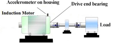
In this section, the motor bearing experimental data supplied by Case Western Reserve University [30] is employed to test the effectiveness of our method. The ball bearing was installed in the driven end of an induction motor and the experimental set-up is shown in Fig. 7. Besides the induction motor, there are a dynamometer, a load mechanism and a tri-axial accelerometer. The dataset contains four bearing health conditions under a certain load: normal condition (NC), inner race fault (IF), roller fault (RF) and outer race fault (OF). The sampling frequency was 12 kHz. We collect 100 samples from each health condition, where each sample contains 1200 data points.

Fig. 7A schematic of the experimental system

4.2.2. Diagnosis results

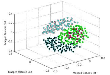
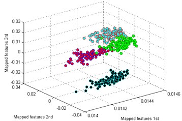
The process procedure of each sample is the same as the above experiment. We also randomly select 10 % samples from each health condition to train the sparse filtering model and then use the rest samples to calculate the learned features. The learned feature vectors of each health condition by sparse filtering are shown in Fig. 8. And the classification result by our method is shown in Fig. 9(a). It is seen that $t$ -SNE also shows its excellent ability in clustering, the features of each fault type are clustered into a ball and can be easily distinguished.

Fig. 8Learned feature vectors of bearing

a) NC

b) IF

c) RF

d) OF

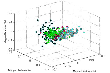
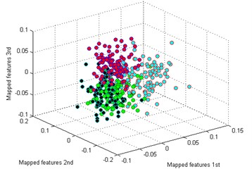
Then we use the other five methods to process the bearing dataset as above. The results are shown in Fig. 9(b)-(f). By comparing the results of the six methods, it is also easy to see that the classification by $t$ -SNE is the best. In Fig. 9(b), although the mapped features by PCA are well performed, several features of each type are not well gathered which is not good as $t$ -SNE. The mapped features by SM are shown in Fig. 9(c), it is noticed that the distance between each type is still too small for distinction. In Fig. 9(d), it shows the mapped features by LPP. It can be seen that parts of the mapped features of NC, IF and RF are mixed together. In Fig. 9(d), which display the mapped features by LPP. It can be observed that most of the mapped features are mixed together. And the mapped features by SPE are shown in Fig. 9(f) which also has several features mixed with each other.

Finally, we employ softmax regression to test the accuracies of the six method, and the process is the same as above. The diagnosis results are showed in Fig. 10 and the average testing accuracies are displayed in Table 3. It is exhibited that the accuracies of $t$ -SNE and PCA are all 100 %, but we should note that the visualization of PCA in Fig. 8(b) is not so well as $t$ -SNE in Fig. 8(a). And the accuracies of the rest methods are also the same as the performances in Fig. 9. Through the above analysis, it is also concluded that the proposed method delivers the optimal performance for the bearing dataset.

Fig. 9Visualize features of bearing

a) T-SNE

b) PCA

c) SM

d) LPP

e) LDA

f) SPE

Table 3Average testing accuracy of bearing using the six methods

Methods	T-SNE	PCA	SM	LPP	LDA	SPE
Accuracy	100 %	100 %	99.22 %	95.97 %	63.56 %	92.64 %

5. Conclusions

An automatic feature extraction method was proposed and implemented to pinpoint the mechanical faults in this paper. In the method, sparse filtering and $t$ -SNE were combined to determine the health conditions in an unsupervised way. By the both of gearbox and bearing experimental cases, it is demonstrated that the proposed method has the strong ability in feature extraction and classification. And also, the proposed method showed its superiority by comparing with other methods.

Fig. 10Diagnosis results of 20 trials of bearing using the six methods

This paper provides the main contributions as follows. Firstly, the proposed method could adaptively learn the features from the raw vibration signals in an intelligent way, which makes it less dependent on the manpower and prior knowledge. Secondly, $t$ -SNE is selected as the dimensionality reduction tool to achieve visualization, which makes the diagnosis results more intuitive. So, the hybrid method of sparse filtering and $t$ -SNE could be an effective automatic feature extraction method for fault diagnosis. At the same time, the proposed method can serve as a reference for fault diagnosis of some other rotating machines.

References

Jiang X., Li S., Wang Y. A novel method for self-adaptive feature extraction using scaling crossover characteristics of signals and combining with LS-SVM for multi-fault diagnosis of gearbox. Journal of Vibroengineering, Vol. 17, Issue 4, 2015, p. 1861-1878.

Search CrossRef
Li Y., Liang X., Xu M., et al. Early fault feature extraction of rolling bearing based on ICD and tunable Q-factor wavelet transform. Mechanical Systems and Signal Processing, Vol. 86, 2017, p. 204-223.

Publisher
Yin J., Wang W., Man Z., Khoo S. Statistical modeling of gear vibration signals and its application to detecting and diagnosing gear faults. Information Sciences, Vol. 259, Issue 3, 2014, p. 295-303.

Publisher
Li W., Zhu Z., Jiang F., Chen G. Fault diagnosis of rotating machinery with a novel statistical feature extraction and evaluation method. Mechanical Systems and Signal Processing, Vol. 50, Issue 51, 2015, p. 414-426.

Publisher
Li Y., Xu M., Wang R., et al. A fault diagnosis scheme for rolling bearing based on local mean decomposition and improved multiscale fuzzy entropy. Journal of Sound and Vibration, Vol. 360, 2016, p. 277-299.

Publisher
Li Y., Xu M., Wei Y., et al. An improvement EMD method based on the optimized rational Hermite interpolation approach and its application to gear fault diagnosis. Measurement, Vol. 63, 2015, p. 330-345.

Publisher
Ming A., Zhang W., Qin Z., Chu F. Envelope calculation of the multi-component signal and its application to the deterministic component cancellation in bearing fault diagnosis. Mechanical Systems and Signal Processing, Vol. 50, Issue 51, 2015, p. 70-100.

Publisher
Monica A. Analysis of induction motor fault diagnosis with fuzzy neural network. Applied Artificial Intelligence, Vol. 17, Issue 2, 2003, p. 105-133.

Publisher
Su H., Chong K., Kumar R. Vibration signal analysis for electrical fault detection of induction machine using neural networks. International Symposium on Information Technology Convergence, Vol. 20, Issue 2, 2007, p. 183-194.

Publisher
Yang J., Yu K., Gong Y., Huang T. Linear spatial pyramid matching using sparse coding for image classification. CVPR, 2009, p. 1794-1801.

Search CrossRef
Le Q., Zou W., Yeung S., Ng A. Learning hierarchical spatio-temporal features for action recognition with independent subspace analysis. CVPR B, Vol. 42, Issue 7, 2011, p. 3361-3368.

Publisher
Lee H., Largman Y., Pham P., Ng A. Unsupervised feature learning for audio classification using convolutional deep belief networks. NIPS, 2009, p. 1096-1104.

Search CrossRef
Amar M., Gondal I., Wilson C. Vibration spectrum imaging: A novel bearing fault classification approach. IEEE Transactions on Industrial Electronics, Vol. 62, Issue 1, 2015, p. 494-502.

Publisher
Cheriyadat A. Unsupervised feature learning for aerial scene classification. IEEE Transactions on Geoscience and Remote Sensing, Vol. 52, Issue 1, 2014, p. 439-451.

Publisher
Chopra P, Yadav S. Fault detection and classification by unsupervised feature extraction and dimensionality reduction. Complex and Intelligent Systems, Vol. 1, Issues 1-4, 2016, p. 1-9.

Publisher
Liu H., Liu C., Huang Y. Adaptive feature extraction using sparse coding for machinery fault diagnosis. Mechanical Systems and Signal Processing, Vol. 25, Issue 2, 2011, p. 558-574.

Publisher
Ajami A., Daneshvar M. Data driven approach for fault detection and diagnosis of turbine in thermal power plant using independent component analysis (ICA). International Journal of Electrical Power and Energy Systems, Vol. 43, Issue 1, 2012, p. 728-735.

Publisher
Hyvarinen A., Hurri J., Patrick O. Natural Image Statistics: A Probabilistic Approach to Early Computational Vision. Computational Imaging and Vision, Springer, London, 2009.

Publisher
Ngiam J., Chen Z., Bhaskar S., Koh P., Ng A. Sparse filtering. Proceedings of Neural Information Processing Systems., 2011, p. 1125-1133.

Search CrossRef
Laurens V., Hinton G. Visualizing Data using t-SNE. Journal of Machine Learning Research, Vol. 9, Issue 2605, 2008, p. 2579-2605.

Search CrossRef
Gisbrecht A., Mokbel B., Hammer B. Linear basis-function t-SNE for fast nonlinear dimensionality reduction. IEEE International Joint Conference on Neural Networks, Vol. 20, 2012, p. 1-8.

Publisher
Hyvärinen A., Oja E. Independent component analysis: algorithms and applications. Neural Networks, Vol. 13, Issue 4, 2000, p. 411-430.

Publisher
Jiang X., Li S., Wang Y. Study on nature of crossover phenomena with application to gearbox fault diagnosis. Mechanical Systems and Signal Processing, Vol. 83, 2016, p. 272-295.

Publisher
Lei Y., Jia F., Lin J., Xing S., Ding S. An intelligent fault diagnosis method using unsupervised feature learning towards mechanical big data. IEEE Transactions on Power Electronics, Vol. 63, Issue 5, 2016, p. 31-37.

Publisher
Yin S., Steven X., Naik A., et al. On PCA-based fault diagnosis techniques. IEEE Control and Fault-Tolerant Systems, 2010, p. 179-184.

Publisher
Yu J. A nonlinear probabilistic method and contribution analysis for machine condition monitoring. Mechanical Systems and Signal Processing, Vol. 37, Issues 1-2, 2013, p. 293-314.

Publisher
Wang X., Zheng Y., Zhao Z., Wang J. Bearing fault diagnosis based on statistical locally linear embedding. Sensors, Vol. 15, Issue 7, 2015, p. 16225-16247.

Publisher
Prince S., Elder J. Probabilistic linear discriminant analysis for inferences about identity. IEEE Computer Society, 2007, p. 1-8.

Publisher
Agrafiotis D., Xu H., Zhu F., et al. Stochastic proximity embedding: methods and applications. Molecular Informatics, Vol. 29, Issue 11, 2010, p. 758-770.

Publisher
Khashei M., Hamadani A., Bijari M. A novel hybrid classification model of artificial neural networks and multiple linear regression models. Expert Systems with Applications, Vol. 39, Issue 3, 2012, p. 2606-2620.

Publisher
Lou X., Loparo K. Bearing fault diagnosis based on wavelet transform and fuzzy inference. Mechanical Systems and Signal Processing, Vol. 18, Issue 5, 2004, p. 1077-1095.

Publisher

Cited by

Insulator fault feature extraction system of substation equipment based on machine vision

Keruo Jiang | Qiaoqun Xia | Lijun Ma | Xin Xu | Zhipeng Shao

(2022)

Two-Channel Information Fusion Weak Signal Detection Based on Correntropy Method

(2022)

Multi-Frequency Weak Signal Detection Based on Wavelet Transform and Parameter Selection of Bistable Stochastic Resonance Model

Siqi Gong | Shunming Li | Houming Wang | Huijie Ma | Tianyi Yu

(2021)

2021 Global Reliability and Prognostics and Health Management (PHM-Nanjing)

(2021)

Parameter-Adaptive VMD Method Based on BAS Optimization Algorithm for Incipient Bearing Fault Diagnosis

Heng-di Wang | Si-er Deng | Jian-xi Yang | Hui Liao | Wen-bo Li

(2020)

Electromyogram (EMG) based fingers movement recognition using sparse filtering of wavelet packet coefficients

SMITA BHAGWAT | PRACHI MUKHERJI

(2020)

A novel bearing intelligent fault diagnosis framework under time-varying working conditions using recurrent neural network

Zenghui An | Shunming Li | Jinrui Wang | Xingxing Jiang

(2020)

A Stacked Autoencoder-Based Deep Neural Network for Achieving Gearbox Fault Diagnosis

Guifang Liu | Huaiqian Bao | Baokun Han

(2018)

An Intelligent Fault Diagnosis Approach Considering the Elimination of the Weight Matrix Multi-Correlation

Zenghui An | Shunming Li | Jinrui Wang | Weiwei Qian | Qijun Wu

(2018)

About this article

Received

31 October 2016

Accepted

22 January 2017

Published

30 June 2017

SUBJECTS

Fault diagnosis based on vibration signal analysis

DOI

https://doi.org/10.21595/jve.2017.17906

Keywords

fault diagnosis

automatic feature extraction

sparse filtering

t-SNE

Acknowledgements

This work was supported by National Natural Science Foundation of China (51675262), Funding of Jiangsu Innovation Program for Graduate Education (KYLX16_0329), the Fundamental Research Funds for the Central Universities (NZ2015103) and the Project of National Key Research and Development Plan of China “New Energy-Saving Environmental Protection Agricultural Engine Development” (2016YFD0700800).

This is an open access article distributed under the Creative Commons Attribution License, which permits unrestricted use, distribution, and reproduction in any medium, provided the original work is properly cited.

Previous article in issue Previous Next article in issue Next

Research article

2020 02 15

A new fault diagnosis method using deep belief network and compressive sensing

Yunfei Ma, Xisheng Jia, Huajun Bai, Guanglong Wang, Guozeng Liu, Chiming Guo

Research article

2019 11 15

Novel complete ensemble EMD with adaptive noise-based hybrid filtering for rolling bearing fault diagnosis

Xiaojun Song, Hongwei Sun, Liwei Zhan

Research article

2018 12 31

An intelligent fault diagnosis method of rotating machinery using L1-regularized sparse filtering

Weiwei Qian, Shunming Li, Jinrui Wang, Zenghui An, Xingxing Jiang

Research article

2017 11 15

Feature reconstruction based on t-SNE: an approach for fault diagnosis of rotating machinery

Jiayu Chen, Dong Zhou, Chuan Lyu, Chen Lu

J. Wang, S. Li, X. Jiang, and C. Cheng, “An automatic feature extraction method and its application in fault diagnosis,” Journal of Vibroengineering, Vol. 19, No. 4, pp. 2521–2533, Jun. 2017, https://doi.org/10.21595/jve.2017.17906

Copy Extrica

Copied to clipboard!

TY  - JOUR
DO  - 10.21595/jve.2017.17906
UR  - https://doi.org/10.21595/jve.2017.17906
TI  - An automatic feature extraction method and its application in fault diagnosis
T2  - Journal of Vibroengineering
AU  - Li, Shunming
AU  - Wang, Jinrui
AU  - Jiang, Xingxing
AU  - Cheng, Chun
PY  - 2017
DA  - 2017/06/30
PB  - JVE International Ltd.
SP  - 2521-2533
IS  - 4
VL  - 19
SN  - 1392-8716
ER  - 

Copy Ris

Copied to clipboard!

@article{Li_2017,
	doi = {10.21595/jve.2017.17906},
	url = {https://doi.org/10.21595/jve.2017.17906},
	year = 2017,
	month = {jun},
	publisher = {{JVE} International Ltd.},
	volume = {19},
	number = {4},
	pages = {2521--2533},
	author = {Shunming Li and Jinrui Wang and Xingxing Jiang and Chun Cheng},
	title = {An automatic feature extraction method and its application in fault diagnosis},
	journal = {Journal of Vibroengineering}
}

Copy Bibtex

Copied to clipboard!

[1]S. Li, J. Wang, X. Jiang, and C. Cheng, “An automatic feature extraction method and its application in fault diagnosis,” Journal of Vibroengineering, vol. 19, no. 4, pp. 2521–2533, Jun. 2017, doi: 10.21595/jve.2017.17906.

Copy IEEE

Copied to clipboard!

Li, Shunming, Jinrui Wang, Xingxing Jiang, and Chun Cheng. “An Automatic Feature Extraction Method and Its Application in Fault Diagnosis.” Journal of Vibroengineering 19, no. 4 (June 30, 2017): 2521–33. https://doi.org/10.21595/jve.2017.17906.

Copy Chicago

Copied to clipboard!

An automatic feature extraction method and its application in fault diagnosis

Abstract

1. Introduction

2. Theoretical background

2.1. Sparse filtering

2.2. T-SNE

3. Proposed framework

4. Fault diagnosis using the proposed method

4.1. Case 1. Gearbox experiment verification

4.1.1. Data description

4.1.2. Diagnosis results

4.2. Case 2. Bearing experiment verification

4.2.1. Data description

4.2.2. Diagnosis results

5. Conclusions

References

Cited by

About this article

Related Articles