Model shape correction method for high-frequency force balance technique

2.1. Mode shape correction factor for translational modes

In general, the first sway mode in the horizontal direction can be formulated as:

where $z$ is the height of current place, $h$ is the total height of the building and $\beta$ is the exponent depending on the actual mode shape. The power spectral density of the generalized force can be expressed as:

where $n$ denotes frequency, $C_0\left(z_1,z_2,n\right)$ is the co-spectrum of fluctuating wind forces which can be expressed as:

where $S_f\left(n\right)$ is the fluctuating wind force spectrum at the standard height, $R\left(z_1-z_2,n\right)$ is the coherence function in terms of the distance between $z_1$ and $z_2$, and $W\left(z\right)$ is the adjusting factor at the height of $z$ as:

where $\alpha$ is the power law for the terrain, and $\nu$ is a constant for different wind case. According to the suggestion of Boggs and Peterka (1989), the value of $\nu$ is taken as 1 for the longitudinal wind case and 2 for lateral or torsional wind cases [6]. The mode shape correction factor is defined as the ratio of the generalized force spectrum for the real mode shape to that for the linear mode shape as:

For a low correction level, the correlation of wind loads falls off rapidly with the increasing distance $\left|z_1-z_2\right|$, therefore, the cross-correlation function $R\left(z_1-z_2,n\right)$ can be assumed to take the form as:

For along wind responses:

For crosswind or torsional responses:

For a high correlation level, a full correlation is assumed for the cross-correlation over the distance between $z_1$and $z_2$:

For along wind response:

For crosswind response:

Fig. 1Mode shape correction factor for high and low correlation assumptions

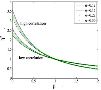
a) Along wind

b) Crosswind

Fig. 1 shows the relation between the mode shape correction factor and the mode shape exponent for different terrains. The mode shape correction method described above has at least two problems. Firstly, the mode shape correction formulae given by Eqs. (7-11) are intended for two extreme cases: full correlation or no-correlation. Actually, the correlation of the wind forces on different levels of tall buildings usually decreases over the distance in a power law manner [9]. Neither the full correlation assumption nor the no-correlation assumption is consistent with the real situation. On the other hand, when investigating the wind effects on an actual tall building, the full wind angle cases should be considered. In wind tunnel tests, the data for 24 or 36 uniformly distributed wind direction angles are commonly measured and then the wind-induced vibrations are analyzed. This means that besides the along wind and crosswind angles, other cases that wind blows obliquely to the building need to be analyzed as well. It’s difficult to discern if such cases belong to the along wind cases or crosswind cases. Consequently, Eqs. (7-11) cannot be applied directly to these cases.

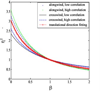
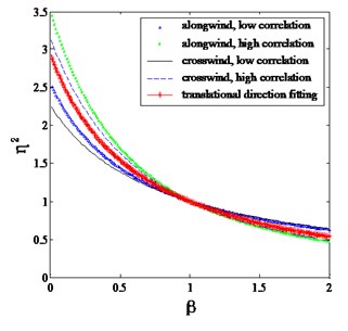
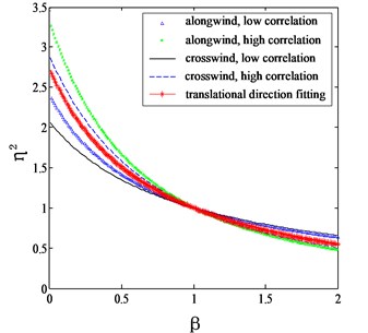
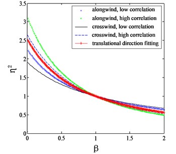
In this study, a uniform correction formula for translational vibration analysis of any wind angles is proposed by referring the form of Eq. (11) as:

The coefficients $a_1$, $a_2$, $a_3$ and $a_4$ must satisfy Eq. (1) for any value of $\alpha$, ${\eta }^2$ should be equal to 1 when $\beta$ equals to 1, and Eq. (2) the correction factor given by Eq. (12) falls intermediately in the correction factor curves given by Eq. (11). Obviously, the former can be automatically satisfied, and the second condition requires repeatedly adjusting the four coefficients to make the computed correction factor falling between the curves of high and low correlation cases for any values of $\alpha$ and $\beta$. In this regard, the four coefficients can only be obtained empirically, any coefficients that satisfy the aforementioned two conditions are acceptable. The final form of Eq. (12) we suggest for practical use is:

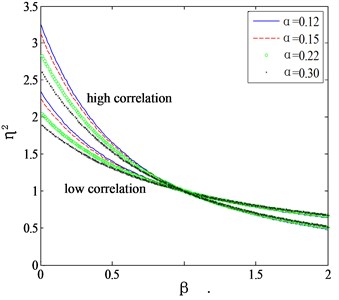
Fig. 2 shows the comparison of the proposed correction factors with those given by Eqs. (7-11). It can be seen that for both the along wind and crosswind cases, the computed correction factors are located between the curves determined by high correlation and low correlation assumptions. Holmes (1987) proposed an intermediate function without considering the category of terrain as:

Fig. 2Proposed mode shape correction factors for different categories of terrains

a)$\alpha =$ 0.12

b)$\alpha =$ 0.15

c)$\alpha =$ 0.22

d)$\alpha =$ 0.30

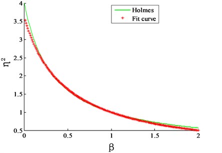
By assuming the wind flow field being uniform over height, a comparison is made between the correction factors proposed by Holmes and this study, as shown in Fig. 3. It can be seen that in the practical range of $\text{0.5}\le \alpha \le \text{2}$, the correction factor proposed in this study shows a good agreement with the results of Holmes. Moreover, the proposed method in this study can take the power law of terrain into consideration.

Fig. 3Comparison of correction factor proposed in this study and by Holmes in 1987

Based on the mode shape correction factor for the generalized forces, the correction factor of the generalized acceleration response can be easily deduced by assuming the mass of each floor being constant, as shown in Eq. (15):

In which:

where $m^{*}$ and $m_1^{*}$ are the modal masses for a real mode shape and assumed linear mode shape, respectively. In a similar way, the mode shape correction factor for the resonant overturning base moment response can be formulated as:

If $\alpha$ and $\beta$ are taken as 0.22 and 1.5, respectively, the value of ${\eta }_M$ is 0.94, indicating that the computed overturning base moment response is not sensitive to the mode shape correction. In other words, the mode shape correction can be ignored when computing the wind-induced overturning base moment response.

2.2. Mode shape correction factor for torsional modes

Wind-induced torsional forces acted on tall buildings are caused by unsymmetrical wind pressure distributed on the building surface. In a similar way as before, the correction factor for the generalized torque can be deduced as

where $S_T\left(n\right)$ and $S_{T_1}\left(n\right)$ are the generalized torque for the real mode shape and assumed mode shape of $\beta =\text{0}$, respectively. For a low correlation level, the correction factor for the generalized torque can be deduced as:

For a high correlation level, the corresponding correction factor is:

Fig. 4 gives the torsional mode shape correction factors for the high and low correlation cases.

Fig. 4Torsional mode shape correction factors for high and low correlation cases

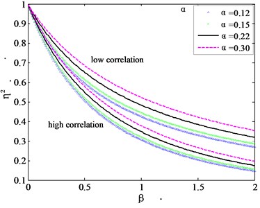
Xu et al. (1993) suggested that the mode shape correction factors for the low correlation case can be used for practical applications [8], but Fig. 4 clearly shows that such a treatment would overestimate the mode correction factor. As before, here an intermediate mode correction factor is proposed for the generalized force in the torsional direction as Eq. (20):

and the corresponding plots are shown in Fig. 5.

It can be seen from Fig. 5 that Eq. (20) is capable of giving appropriate corrections of torsional modes for different terrains. If $\alpha$ is taken as zero, referring to a uniform flow field case, the mode shape correction factor given by Eq. (20) is exactly the same as suggested of Holmes. Li et al. [10] proposed a formula for estimating the mode shape correction factor of torsional modes as:

Tallin and Ellingwood [11] in 1985 carried out an experimental study on the value of mode shape correction factors. By assuming that $\alpha$ equals to zero, the torsional mode shape correction factors estimated by this study and the one from the study of Li are compared to the experimental results given by Tallin and Ellingwood, as shown in Table 1. It can be seen that the torsional mode shape correction factor given by this study is closer to the experimental results, which demonstrates the applicability of Eq. (20).

Fig. 5Mode shape correction factors for torsional generalized force

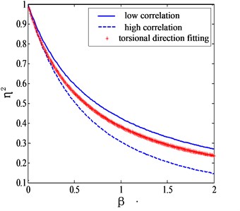
a)$\alpha =\text{0.12}$

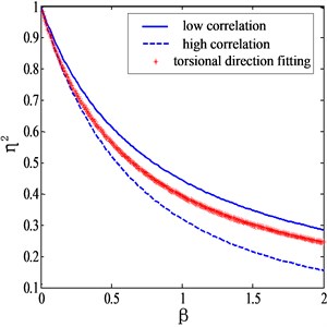
b)$\alpha =\text{0.15}$

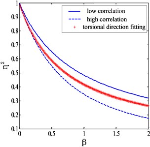
c)$\alpha =\text{0.22}$

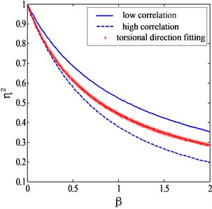
d)$\alpha =\text{0.30}$

In a similar way like the procedure of obtaining the correction factor of the acceleration response for the sway modes, the correction factor for the acceleration response in torsional direction can be easily deduced as:

where:

in which $m^{*}\text{,}$$m_1^{*}$ are the modal masses for the real mode shapes and ideal linear modes, respectively.

The mode shape correction factors for resonant base overturning moment response can subsequently be deduced based on the concept of inertia force as:

Substituting a pair of normally used value of $\alpha$ and $\beta$, for instance 0.22 and 0.15 respectively, into Eq. (23), the mode shape correction factor is obtained as equal to about 0.83, meaning that the effect of mode shape on the base torsional moment response cannot be ignored.

2.3. Mode coupling effects

As it is known to researchers and engineers, the classic HFFB theory ignores the mode correlation effect. This treatment is applicable for buildings and structures with a simple structural system and low mode coupling effects. However, as the development of building techniques, more and more modern super-tall buildings with the complex structure system have coupling modes. Ignoring the mode coupling effect would lead to unreliable computational results of wind-induced vibration. In this section, the mode coupling effects on structural response are discussed. Here only the first mode in each direction (two sway directions along the orthogonal horizontal axes and one torsional direction along the vertical axis) are considered.

The power spectral density of the modal force can be formulated in Eq. (24) by neglecting the item of co-spectrum.

where ${\eta }_{1x}$, ${\eta }_{1y}^2$ and ${\eta }_{1\theta }^2$ are the mode shape correction factors for the modal force $F_1$ in the direction of $x$, $y$ and $\theta$, and so on. The method described in Eq. (24) is called method I in this study. In fact, the modal forces can be written in a more accurate form as:

Unlike Eq. (24), Eq. (25), called method II, took the co-spectrum into consideration. Obviously, Eq. (25) took the mode shape correction and the mode coupling effect into consideration, and theoretically it is the most accurate form to calculate the spectrum of modal forces. In the next section, the Guangzhou East Tower will be taken as an illustrative example to discuss the computational results using different methods.

3.1. Introduction to Guangzhou east tower

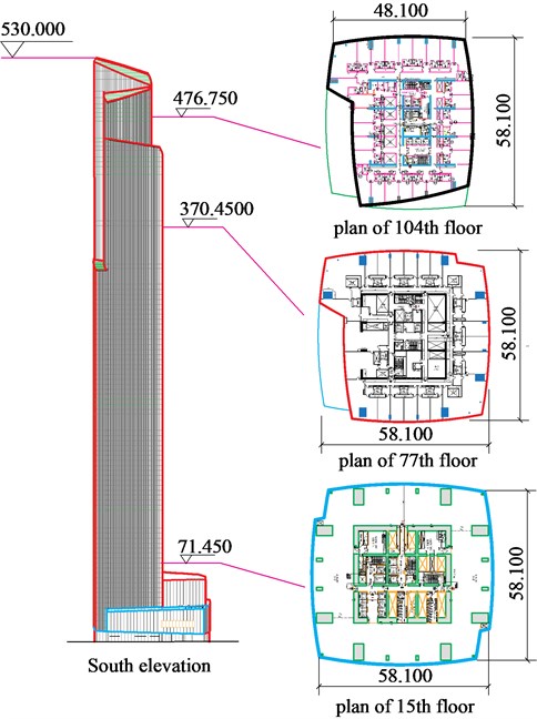
In this section, an iconic super-tall building, the Guangzhou East Tower (GZET), is taken as an example to show the effectiveness of the proposed mode shape correction factors and discuss the mode coupling effect. The GZET has the hight of 530 m above ground and is now the tallest building in Guangzhou, China. Guangzhou, located in the southeast coastal region of China, is one of the regions most seriously affected by strong typhoons. Hence, the GZET could endure wind effects induced by typhoons and can be regarded as ideal examples for investigating typhoon effects on super-tall buildings. The architectural design of GZET adopted a so-called ‘set-back’ scheme in the upper part of the building to reduce its response to strong wind. Its elevation and typical plan are illustrated in Fig. 6.

Fig. 6Elevation and typical planes of GZET (unit: m)

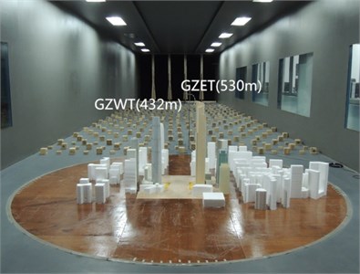
A rigid model with a geometric length scale of 1:500 was made to represent the GZET. The model was made of balsa and foam, and was mounted on a metal slab which was rigidly connected to a high-frequency force balance (HFFB). The models of surrounding buildings that might affect the wind effects on the tested building were also made and mounted on the ground of the wind tunnel to simulate the surrounding conditions. Fig. 7 shows the models mounted in the wind tunnel. A Pitot tube was installed at height of GZET model (1.06 m above the wind tunnel ground) to measure the reference wind speed. The wind direction was defined as an angle $\beta$ from the east along an anti-clockwise direction varied from 0° to 360° with the increment of 10°. In the wind tunnel test, the forces at the bases of the building model were measured by an ATI-type HFFB. The ATI-type HFFB is capable of measuring six force components including the shear forces along two horizontal directions, axial force along the vertical direction, bending moment along two horizontal directions and torque along the vertical direction. The building model of GZET was installed on the ATI force balances by ensuring that the coordinate system of the building matched the coordinate system of the balance. The sampling frequency was set as 400 Hz with the sampling length of 40960 for each wind direction.

Fig. 7Simulated mean wind speed and turbulence intensity profile in the wind tunnel

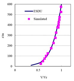
a) Mean wind speed

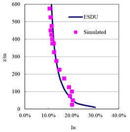
b) Turbulence intensity

Fig. 8Models in wind tunnel

3.2. Results and discussions

3.2.1. Power spectrum of modal forces

The properties of the modal force on a structure can significantly affect its response. Here the spectrum of modal forces computed by the classic HFFB method, the method considering the mode shape correction factors and the method considering the mode coupling effects using method I, is presented here in Fig. 9. It can be seen that, if the mode coupling effect is ignored, the computed power spectrum of modal forces changed a little bit when the mode shape correction factor was considered. Actually, the computed mode shape correction factor is about 0.7 for this case, meaning that it’s necessary to make the mode shape correction before computing the structural response. On the other hand, the mode shape coupling effect is significant for the wind direction of 0°, indicating that the effect of modal shape coupling effect on the structural response should not be ignored.

Fig. 10 gives the spectrum of modal force computed by the method I and II. The result computed by the classic HFFB method without considering the mode shape correction and mode coupling effect is also given as a reference. It can be seen that spectrum computation results are close to each other in the wind direction of 0°, whereas in the wind direction of 90°, the results obtained by method I and II are quite different from the spectrum computed by the classic HFFB method. This means that it’s necessary to carry out the mode shape correction and consider the mode coupling effect when estimating the wind-induced response. The difference of the results given by method I and II cannot be clearly identified through Fig. 10, and it will be discussed in the next section.

Fig. 9Comparison of computed power spectrum of modal force using different methods

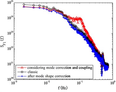
a) 0°

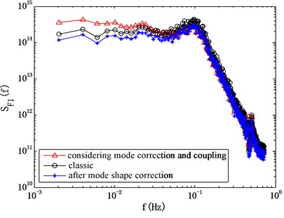
b) 90°

Fig. 10Comparison of results given by method I and II

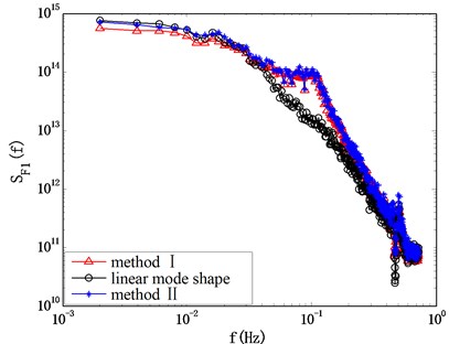
a) 0°

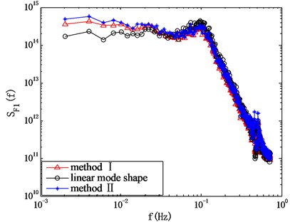
b) 90°

3.2.2. Displacement response

Displacement is usually the basic variable in the dynamic equation. In this section, the structural displacement response is computed to investigate the influence of the co-spectrum item in Eq. (25). Fig. 11 shows the displacement at the top of GZET under all wind directions. It can be seen that the displacements given by method I and II are different. In most of wind direction cases, the results given by method II, which considered the co-spectrum item, are greater than that given by method II. For instance, under the wind direction of 100°, the displacement given by method II is about 13.4 % greater than that given by method I. For the case of GZET, the mode coupling effect is significant and considering the co-spectrum item might tend to provide more safety to the structure.

The significant mode coupling effect for this case can be attributed to the drift angle between the geometry axes and the modal vibration direction, as shown in Fig. 12. Just as aforementioned, the axes of ATI balance matched the geometrical axes at the wind tunnel test, therefore, the wind tunnel test and the subsequent wind-induced response analysis are based on the geometrical coordinate system. For common super-tall buildings, the modal vibration directions for the first two modes are usually consistent with two horizontal geometrical axes. However, there is an obvious drift angle of 32.6° between the geometrical axes and the modal vibration directions for the first two modes. In other words, the modal vibrations for the first two modes project components on both the geometrical axes of $x$ and $y$. Therefore, the mode coupling effect is significant. Since the unsymmetrical structural system became more and more popular in modern super-tall building construction, the mode coupling effect of these buildings might be more obvious than those built in the past, and consequently, the mode coupling effect should be taken into consideration when estimating their wind-induced vibrations.

Fig. 11Displacement response computed by method I and II

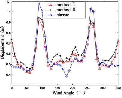
a) Direction $x$

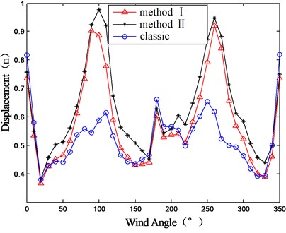
b) Direction $y$

Fig. 12drift angle between geometrical axes and modal vibration direction

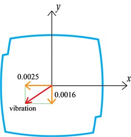
a) First order

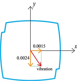
b) Second order