Evaluation and numerical simulation of soil type effects on seismic soil-structure interaction response of RC structures

1. Introduction

Although seismic waves travel mainly through rock in their course to the ground surface, the last portion of that propagation is often through soil, and the characteristics of the soil can greatly influence the nature of shaking at the ground surface [1]. Based on many previous researches, it is recognized that considering the SSI may significantly affect the response of the structure to the earthquake. The SSI affects different structures differently; it depends on the characteristics of the structure, the soil, and the earthquake record. In some circumstances, the effect could be ignored, but it could prove highly significant in other cases. Since accounting for SSI effects entails following an inherently complicated procedure, SSI effects are ignored in the majority of design codes, presuming that the inattention to soil-structure interaction yields conservative results [2]. The presumption “neglecting the SSI gives conservative results” is not always valid, and the SSI may even considerably increase the responses of structures at times [3]. Accordingly, it seems more appropriate to take the SSI effect into account; one would also benefit from the effect if it introduces a conservative change. In fact, the subsoil provides a flexible base, reduces the stiffness, and increases the deformations and damping [4]. On the other hand, it could affect the frequency content of the incoming seismic motions.

The effect of local soil and geologic conditions on the intensity of ground shaking and earthquake damage has been known for many years. MacMurdo [5] noted that “buildings situated on rock were not by any means affected as much as those whose foundations did not reach the bottom of the soil” in the 1819 earthquake in Cutch, India. Mallet [6], in his report on the 1857 Neapolitan earthquake, reported the effect of local geologic conditions on structural damage. Many researchers have studied the behavior of structures supported on shallow foundations; Chopra and Yim [7], modeled the behavior of shallow foundations using Winkler springs. They concluded that taking the SSI effect into account causes a reduction in the moment demand of the structures. ATC 40 [8] believes that stiff and strong foundations do not always surpass flexible and weak foundations; in fact, flexible foundations increase the deformation, leading to a drop in the demands. Spyrakos et al studied the SSI effect on base isolated buildings [9], concluding that the SSI effects for squat structures founded on low-stiffness soil stratum are deeply significant. Zhang and Tang [10] demonstrated that ductility demands may dramatically increase in case of a compliant foundation. The SSI effect on the seismic behavior of multi degree-of-freedom (MDOF) systems was assessed by Dutta et al [11] and Barcena and Esteva [12]. Tang and Zhang performed a comprehensive probabilistic seismic demand analysis of shear walls considering the SSI effect [13]. Many other researches such as Raychowdhury and Prishati [14], Ganjavi and Hao [15, 16] and Abedi-Nik and Khoshnudian [17] have been done on the SSI effect. Afterwards, Ganjavi, Hao and Hajirasouliha [18] underlined the importance of higher modes for soil-structure systems in comparison with fixed based structures. Soil-underground structure static and dynamic interaction was studied by Haiyang [19]. Some researchers tried to compare the experimental observations with the analytical results obtained while taking the SSI into account; examples include [20, 21] and [22]. The role of SSI effect on isolated structures was studied by Tsai and Hsueh [23]. Examining the effects of soil-structure interaction on the deflection modification factor of buildings was another interesting subject that captured the attention of researchers such as Abedi-Nik and Khoshnoudian [24].

As noted above, not all of the findings produced in the previous researches are consonant with each other; some of them are even contradictory. All of them have argued for the strong effect of SSI on the behavior of structures, but arrived at different conclusions about the variations in the structural behavior. Therefore, these investigations fail to provide any conclusive evidence on the way the structural responses are affected by the soil type. This discrepancy in the conclusions is very likely due to the fact that the structures and soil types studied were all different. This is the reason why the present research covers disparate structures and soil types. The results of the present study and those of the previous studies fit together for sandy soils but not for soft clay soils.

2. Characteristics of concrete frames, soil and earthquake records

Geometric and material nonlinearity in the superstructure, the foundation and the soil could cause some nonlinearity in soil-structure systems. The nonlinearity may originate from diverse phenomena such as: 1) yielding of seismic-force-resisting elements in the superstructure; 2) yielding of soil, 3) gapping between the foundation and soil, which tends to occur in situations such as base uplift or separation of foundation sidewalls from the surrounding material; and 4) yielding of foundation elements [25]. Most of the researches conducted on nonlinear SSI behavior have assumed either a nonlinear structure with a linear/equivalent-linear soil or a linear structure with a soil capable of yielding.

The literature on the subject shows that material and geometric nonlinearities in the soil may be beneficial to the seismic response of a structure. In order to dissipate the energy and protect the structure, Gajan and Kutter [26] suggested revising the foundation design strategy by allowing for significant yielding within either the foundation or the immediate soil in the vicinity of the foundation.

In the present paper it is intended to consider the likely scenario. For this reason, the soil and the structure are both assumed to be nonlinear. The 2D nonlinear analytical models of soil-structure systems were developed for the nonlinear dynamic analysis with OpenSEES software [27].

2.1. Characteristics of the frames

In the present study, five planar concrete moment resisting frames are examined. The frames have 3 bays and 3, 6, 9, 12 and 15 stories. The bay length and the story height are 5 and 3 meters respectively. The moment resisting concrete frames have been designed with a peak ground acceleration (PGA) value equal to 0.35g and class B soil according to INBR-6 (Iranian National Building Regulations, Section 6). The dead load on the beams is assumed to be 24500 N/m plus the self-weight of the beams, and the live loads on the beams are assumed to be 9800 N/m. The yield stress of the bar material is equal to 4×10⁸ Pa, and the concrete strength is assumed to be 25×10⁶ Pa. The material constitutive models are presented in Fig. 1. The second-order effects are accurately accounted for through the formulation of large displacements. For the confined and unconfined concrete constitutive models, the Kent-Scott-Park model [28] is employed. The constitutive parameters of this model are shown in Fig. 1 and explained below:

Fig. 1Material constitutive models: fc – concrete peak strength in compression [Pa], fu – residual strength [Pa], ε0 – strain at peak strength [%], εu – ultimate compressive strain [%]

a) Concrete

b) Steel

The cover and core concrete in the column cross-sections are considered as unconfined and confined concrete respectively. The confined concrete stress-strain relationships are extracted from Saatcioglu and Razvi [29]. Paulay and Priestley [30] suggested the ultimate compressive strain of confined concrete as:

1

${\epsilon }_{uc}={\epsilon }_{uo}+1.4\frac{{\rho }_v{f}_{yh}{\epsilon }_{us}}{f_{cc}},$

where ${\epsilon }_{uc}$ – ultimate compressive strain of confined concrete [%], ${\epsilon }_{uo}$ – ultimate compressive strain of unconfined concrete [%], ${\epsilon }_{us}$ – ultimate strain of reinforcing steel in tensile [%], ${\rho }_v$ – volumetric ratio of confining steel [%], $f_{yh}$ – yield stress of confining steel [Pa], $f_{cc}$ – peak strength of confined concrete in compression [Pa].

The lumped mass matrix of the frames is built by applying the total of dead loads plus 20 % of live loads. The beams and columns are modeled as fiber sections with concrete and reinforcing steel material layers. The characteristics of the cross-sections for columns and beams are illustrated in Tables 1 and 2.

2.2. Soil modeling procedure

In the present paper, the soil layers are modeled using isoperimetric four node quadrilateral finite elements with bilinear displacement interpolation. The finite element mesh size is considered to be 2.0 m in $x$ and $z$ directions. It is assumed that the soil domain is under plane strain conditions with a constant soil thickness equal to the inter-frame distance. The material of the clay soil is modeled using a modified pressure-independent multi-yield-surface model with an associative flow rule, and the yield surfaces are of the Von Mises type. The material of the sandy soil is modeled using a pressure-dependent relation with a non-associative flow rule to reproduce dilatancy effects. The yield surfaces are of the Drucker-Prager type.

Table 1Column section of frames

Column sections
	3 story	6 story	9 story	12 story	15 story
Story 1	0.4×0.4 [m]	0.5×0.5 [m]	0.5×0.5 [m]	0.65×0.65 [m]	0.8×0.8 [m]
Story 2	0.4×0.4 [m]	0.5×0.5 [m]	0.5×0.5 [m]	0.65×0.65 [m]	0.8×0.8 [m]
Story 3	0.4×0.4 [m]	0.4×0.4 [m]	0.5×0.5 [m]	0.65×0.65 [m]	0.8×0.8 [m]
Story 4	–	0.4×0.4 [m]	0.5×0.5 [m]	0.65×0.65 [m]	0.8×0.8 [m]
Story 5	–	0.4×0.4 [m]	0.5×0.5 [m]	0.65×0.65 [m]	0.8×0.8 [m]
Story 6	–	0.4×0.4 [m]	0.4×0.4 [m]	0.5×0.5 [m]	0.6×0.6 [m]
Story 7	–	–×	0.4×0.4 [m]	0.5×0.5 [m]	0.6×0.6 [m]
Story 8	–	–	0.4×0.4 [m]	0.5×0.5 [m]	0.6×0.6 [m]
Story 9	–	–	0.4×0.4 [m]	0.5×0.5 [m]	0.6×0.6 [m]
Story 10	–	–	–	0.4×0.4 [m]	0.5×0.5 [m]
Story 11	–	–	–	0.4×0.4 [m]	0.5×0.5 [m]
Story 12	–	–	–	0.4×0.4 [m]	0.5×0.5 [m]
Story 13	–	–	–	–	0.4×0.4 [m]
Story 14	–	–	–	–	0.4×0.4 [m]
Story 15	–	–	–	–	0.4×0.4 [m]

Table 2Beam section of frames

Beam Sections
Story 1	3 story	6 story	9 story	12 story	15 story
Story 2	0.3×0.4 [m]	0.4×0.5 [m]	0.4×0.5 [m]	0.45×0.55 [m]	0.5×0.65 [m]
Story 3	0.3×0.4 [m]	0.4×0.5 [m]	0.4×0.5 [m]	0.45×0.55 [m]	0.5×0.65 [m]
Story 4	0.3×0.4 [m]	0.3×0.4 [m]	0.4×0.5 [m]	0.45×0.55 [m]	0.5×0.65 [m]
Story 5	–	0.3×0.4 [m]	0.4×0.5 [m]	0.45×0.55 [m]	0.5×0.65 [m]
Story 6	–	0.3×0.4 [m]	0.4×0.5 [m]	0.45×0.55 [m]	0.5×0.65 [m]
Story 7	–	0.3×0.4 [m]	0.3×0.4 [m]	0.4×0.5 [m]	0.4×0.5 [m]
Story 8	–	–	0.3×0.4 [m]	0.4×0.5 [m]	0.4×0.5 [m]
Story 9	–	–	0.3×0.4 [m]	0.4×0.5 [m]	0.4×0.5 [m]
Story 10	–	–	0.3×0.4 [m]	0.4×0.5 [m]	0.4×0.5 [m]
Story 11	–	–	–	0.3×0.4 [m]	0.3×0.4 [m]
Story 12	–	–	–	0.3×0.4 [m]	0.3×0.4 [m]
Story 13	–	–	–	0.3×0.4 [m]	0.3×0.4 [m]
Story 14	–	–	–	–	0.3×0.4 [m]
Story 15	–	–	–	–	0.3×0.4 [m]

2.2.1. Modeling soil domain boundary

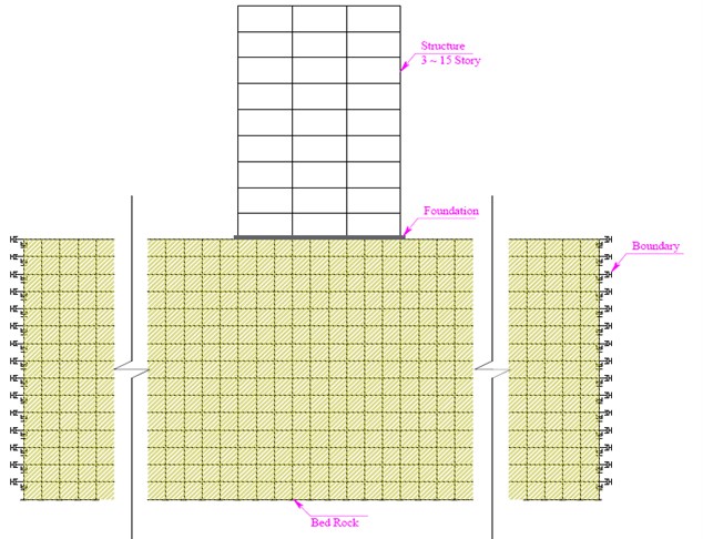
The SSI effects are categorized by FEMA P-750 [31] into inertial interaction effects, kinematic interaction effects, and soil-foundation flexibility effects. On the other hand, the methods that can be used to evaluate the mentioned effects fall into the two categories of direct and substructure approaches. In the direct analysis method, the soil and structure are modeled simultaneously and analyzed as an integrated system. The substructure approach involves dividing the SSI problem into distinct parts that are combined to formulate the complete solution. The superposition inherent in the substructure approach requires making the assumption that the soil-structure system behaves linearly, leading to some error in the results. For this reason, the direct method is the one employed in the present study. Modeling the SSI system for an infinite media entails tackling the problem of modeling domain boundaries. Infinite boundaries have to reflect no waves back into the computational domain and absorb all outgoing waves. Lysmer and Kuhlemeyer [32] proposed the standard viscous boundary which is defined by using Eqs. (2-3):

2

$C_n=\alpha \rho v_p,v_p=\sqrt{\frac{2G(1-\nu )}{\rho (1-2\nu )}},$

3

$C_s=b\rho v_s,\mathrm{}\mathrm{}\mathrm{}\mathrm{}{v}_s=\sqrt{\frac{G}{\rho }},$

where $C_n$ – normal damping [(N×S)/m], $C_s$ – shear damping [(N×S)/m], $\rho$ – mass density of soil [N/m²$]$, $\nu$ – Poisson ratio of soil [%], $v_p$ – propagation velocity of dilatational waves [m/s], $v_s$ – propagation velocity of shear waves [m/s].

In the present study, a single zero length element is used to define the Lysmer-Kuhlemeyer dashpot; one end of the Lysmer-Kuhlemeyer dashpot element is fixed against all displacements, while the other end is assigned a restraint of the type equalDOF with the soil node. Two series of dashpots are needed to introduce this boundary into the model. As depicted in Fig. 2, dashpots are oriented normally and tangentially to the boundary of the finite element mesh. The soil layer height on the bedrock is assumed to be 30 meters, and the length of the soil domain, boundary to boundary distance, is considered to be 100 meters.

Fig. 2Soil medium boundary

The soil layer is characterized by the following parameters: $\rho$ – mass density of soil [N/m³], $G_r$ – low strain shear modulus [Pa], $B_r$ – bulk modulus (At reference mean effective confining pressure) [Pa], $f$ – friction angle at peak shear strength [Deg], $c$ – apparent cohesion at zero effective confinement (For clay) [Pa], ${\gamma }_{max}$ – an octahedral shear strain at which the maximum shear strength is reached [Deg], $P_r$ – reference mean effective confining pressure at which $G_r$, $B_r$ and ${\gamma }_{max}$ are defined [Pa].

The material damping matrix $C$ of the SSI system is constructed using the Rayleigh method [33], through assembling the corresponding damping matrices of the structure and the soil. The factors of proportionality for damping matrices are calculated for 5 % and 10 % viscous damping for the structure and the soil respectively. The nonlinear equations of structural equilibrium are satisfied using the accelerated Newton algorithm based on Krylov subspaces [34]. In the nonlinear time history analysis, the $P$-$\mathrm{\Delta }$ effects are taken into account.

2.2.2. Soil types

Soil deposits tend to act as a filter for seismic waves by attenuating the motion at certain frequencies and amplifying it at others. Since soil conditions often vary dramatically over short distances, levels of ground shaking can vary significantly within a small area. One of the most important aspects of geotechnical earthquake engineering practice involves evaluation of the effects of local soil conditions on strong ground motions [1]. Different soil types affect the structure responses differently. In order to address all kinds of soils, seven types of soils, namely loose, medium, medium dense, dense sand, as well as soft, medium, and stiff clay, are considered in the present study. The water table is considered to be below the soil layer. The characteristics of such soil types are presented in Table 3.

Table 3Characteristics of each soil type

Soil type	Mass density	Shear modulus at low strain	Cohesion at zero confinement	Peak shear strain	Friction angle
Unit	[N/m2]	[N/m2]	[N/m2]	[Deg]	[Deg]
Loose sand	17	550000	0	0.1	29
Medium sand	19	750000	0	0.1	33
Medium dense sand	20	1000000	0	0.1	37
Dense sand	21	1300000	0	0.1	40
Soft clay	13	130000	18	0.1	0
Medium clay	15	600000	37	0.1	0
Stiff clay	18	1500000	75	0.1	0

Having the characteristics of soil layers in Table 3, one can calculate the shear wave velocity of soil layers using Eq. (4) [1], the values of which are presented in Table 4. Knowing the shear wave velocity, one can calculate the soil layer period based on Eq. (5) [1]. In Table 5, the soil layer period values obtained from Eq. (5) are compared with those obtained from the numerical models:

4

$v_s=\sqrt{\frac{G}{\rho }},$

5

$T=\frac{4H}{V_s},$

where $V_s$ – soil shear wave velocity [m/s], $G$ – soil shear modulus [Pa], $\rho$ – soil mass density [N/m³$]$, $H$ – soil layer depth [m], $T$ – soil layer period [s].

Table 4Shear wave velocity

Soil shear wave velocity [m/s$]$
Soil type	${\left(G/\rho \right)}^{0.5}$
Loose sand	179.87
Medium sand	198.68
Medium dense sand	223.61
Dense sand	248.81
Soft clay	100.00
Medium clay	200.00
Stiff clay	288.68

Table 5Comparing the soil layer period from the experimental equation and Opensees models

Period of soil layer [s]			(Period based on the model)/ (Period based on the formula)
Soil type	Based on experimental equation (4H/Vs)	Based on opensees models
Loose sand	0.67	0.48816	1.37
Medium sand	0.60	0.44238	1.37
Medium dense sand	0.54	0.39117	1.37
Dense sand	0.48	0.35155	1.37
Soft clay	1.20	0.86204	1.39
Medium clay	0.60	0.431021	1.39
Stiff clay	0.42	0.29862	1.39

According to Table 5, the period values calculated in the numerical models are consistent with those calculated with the experimental formula.

3. Period lengthening due to SSI effect; comparison between numerical model results and those computed based on NEHRP method

NEHRP Consultant Joint Venture, a joint venture of the Applied Technology Council (ATC) and the Consortium of Universities for Research in Earthquake Engineering (CUREE), published a report in 2012 [25] which attempted to devise a practical method for considering the SSI effect.

According to NEHRP, the SSI effects fall into the three categories of inertial interaction effects, kinematic interaction effects, and soil-foundation flexibility effects. The terms kinematic and inertial interaction were introduced by Kausel [37].

In the present research, the verification and validation of the numerical models are performed with the characteristics presented in NEHRP report.

3.2. Soil-structure system period obtained from NEHRP

NEHRP presents a number of period lengthening graphs which indicate the period lengthening caused by SSI. Such graphs are depicted here in Fig. 3. NEHRP presents the graphs for h/B values equal to 1, 2, and 4 and for $h/B$ values equal to 0.5, 1.5, and 2.5 (corresponding to the frames studied herein), which are generated by interpolation.

The expressions $h/V_{s}T\text{'}$ and h/B are shown in Table 10 and 11 respectively for all frames. According to NEHRP, the most important parameter for controlling the significance of SSI effect is the term $h/V_{s}T\text{'}$ [25], meaning that the higher the value of $h/V_{s}T\text{'}$, the stronger the effect of SSI. As a matter of fact, the term $h/V_{s}T\text{'}$ denotes the structure-to-soil stiffness ratio.

According to Table 10, for a certain soil type, the term $h/V_{s}T\text{'}$ grows with increasing frame height except for the 15 story frame; it is the case for all soil types. This shows that, in the range of low and medium rise buildings, the SSI effects escalate as the structure becomes taller, but for high rise buildings, the SSI effects wear off as the structure becomes taller. NEHRP supports this phenomenon by specifying that “Tall buildings typically have low amounts of $h/V_{s}T\text{'}$ ratio”.

With the help of Fig. 3, Table 10, and Table 11, the period lengthening can be calculated according to the NEHRP method, as presented in Table 12.

By comparing Table 12 with Table 9, it could be inferred that the period lengthening calculated by the numerical models are congruent with those calculated by NEHRP graphs; in this way, the models are verified. Accordingly, the NEHRP admits results 1 and 2 mentioned in part 3.1.

Fig. 3Period lengthening graph, NEHRP. The parameters are as follows: h – structure height [m], B – foundation width [m], L – foundation length [m], T' – structural first mode period [s], T- – soil-structure system period [s], Vs – soil shear wave velocity [m/s]

Table 10h/VsT' for studied frames

	$h/V_{s}T\text{'}$
	3 St	6 St	9 St	12 St	15 St
Loose sand	0.08950	0.10660	0.12126	0.13405	0.13183
Medium sand	0.08103	0.09651	0.10978	0.12136	0.11935
Medium dense sand	0.07199	0.08575	0.09754	0.10783	0.10605
Dense sand	0.06470	0.07707	0.08766	0.09691	0.09531
Soft clay	0.16098	0.19175	0.21811	0.24111	0.23713
Medium clay	0.08049	0.09587	0.10906	0.12055	0.11856
Stiff clay	0.05577	0.06642	0.07556	0.08352	0.08214

Table 11h/B for the studied frames

	$h/B$
3 St	0.5
6 St	1
9 St	1.5
12 St	2
15 St	2.5

Table 12The T-/T' ratio – based on NEHRP

	$\stackrel{-}{T}/T\text{'}$
	3 St	6 St	9 St	12 St	15 St
Loose sand	1.03816	1.05489	1.07302	1.09533	1.10219
Medium sand	1.03160	1.04579	1.06112	1.08007	1.08607
Medium dense sand	1.02512	1.03684	1.04943	1.06506	1.07015
Dense sand	1.02028	1.03017	1.04074	1.05389	1.05825
Soft clay	1.11234	1.15853	1.20931	1.26914	1.28412
Medium clay	1.03120	1.04524	1.06040	1.07915	1.08509
Stiff clay	1.01484	1.02268	1.03100	1.04134	1.04484

4. Effect of local site condition on ground motion

Local site conditions can profoundly affect all of the important characteristics of earthquake such as amplitude, frequency content, and duration of strong motion. The extent of their influence depends not only on the geometry and properties of the subsurface materials, but also on site topography, and the characteristics of input motion [1].

The displacement of soil at the top of the soil layer (ground level) is illustrated in Fig. 4 for various soil types under the action of record number one in Table 6 with PGA = 0.5. As it is seen, the displacement of the top of the soil layer is completely varied for different soil types. As it was expected, the “Soft Clay” has the lowest natural frequency but the largest amplitude of oscillation. On the contrary, “Dense Sand” has the highest value of frequency but the lowest amplitude of oscillation.

Fig. 4Displacement of soil at top of the soil layer (ground level) – PGA = 0.5 g

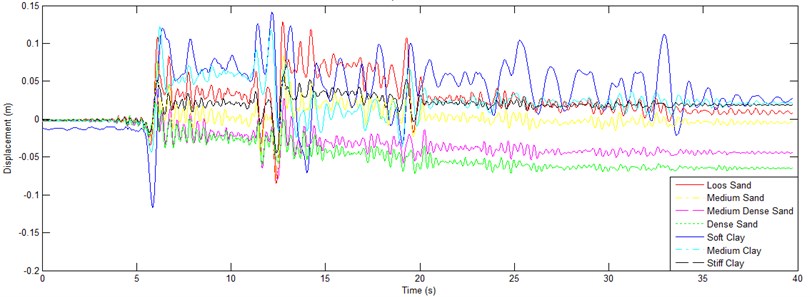
Fig. 5Acceleration of soil at top of the soil layer (ground level) – dense sand – Sc = 0.1 g

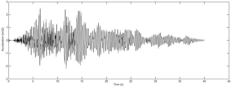
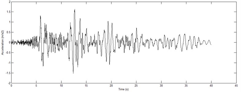
Fig. 6Acceleration of soil at top of the soil layer (ground level) – soft clay – Sc = 0.1 g

Results show that every record changes dramatically in frequency content, PGA, Strong motion duration and other properties after passing through the soil layers; the changes are different for different soil types. According to Fig. 4, the largest value for the displacement of the top of soil layer belongs to soft clay and loose sand.

Fig. 5 and Fig. 6 illustrate the acceleration at the top of the soil layer for “Dense Sand” and “Soft Clay”, representative of the densest and the loosest soil types.

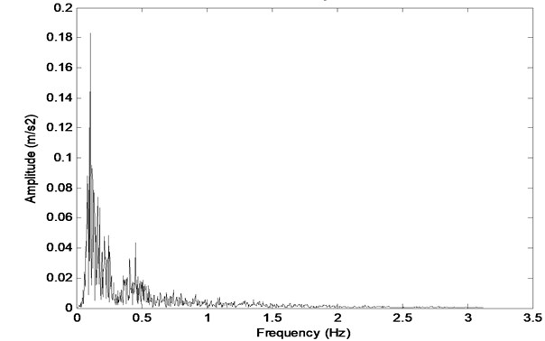
The characteristics of local soil deposits can also affect the extent to which ground motion amplification will occur. This phenomenon can be tracked in Figs. 7 and 8; these figures show the acceleration of the soil top in the frequency domain for dense sand and soft clay respectively. As illustrated in Figs. 7 and 8, softer soils (Soft Clay) amplify low-frequency (long-period) bedrock motion to a greater extent than stiffer soils do. On the contrary, stiffer soils (Dense Sand) amplify high-frequency (low-period) bedrock motion more profoundly than softer soils do.

Fig. 7Acceleration of soil at top of the soil layer (ground level) – dense sand – Sc = 0.1 g

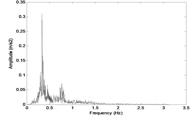
Fig. 8Acceleration of soil at top of the soil layer (ground level) – soft clay – Sc = 0.1 g

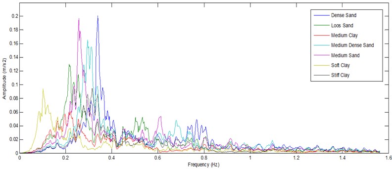
Therefore, it is expected that low rise structure responses would be amplified on dense soils, and high rise structure responses would be amplified on soft soils. The acceleration of top of the soil layer for different soil types is illustrated in Fig. 9.

As shown in Fig. Fig. 9, sandy soils develop larger amplitudes of acceleration in the frequency domain. The predominant frequency of soft clay and dense sand is the smallest and the largest respectively.

Fig. 9Comparison of acceleration on top of soil layer for different soil types under the action of Rec01- Sc = 0.1 g (frequency domain)

5. SSI effect on the Pushover curve

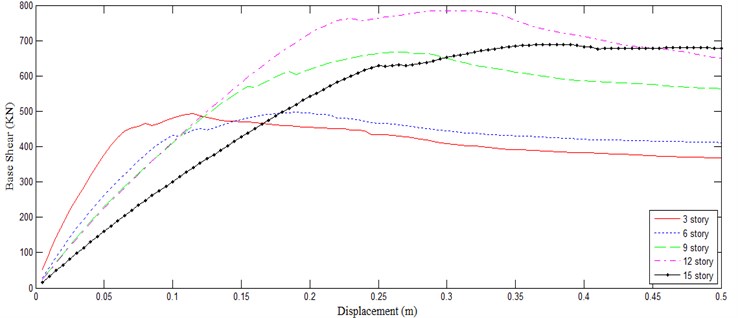
The Pushover (PO) curves of the rigid based frames are shown in Fig. 10. Since PO curves express the static behavior of structures, it is expected that considering the SSI effect doesn’t greatly affect this curve. The PO curves of the 3 and 15 story frames are illustrated in Fig. 11 and Fig. 12 respectively; these figures prove that the effect of SSI on the PO curves is negligible. Similar results were confirmed by other researchers [38]. In these figures, it is clearly evident that the SSI effect is more marked on high rise buildings than low rise ones.

Fig. 10Pushover curve for all structures – rigid based

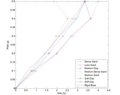
6. Effect of SSI on IDA curve

Subsoil characteristics affect the IDA curve dramatically. As it was discussed earlier, the subsoil attenuates motion at certain frequencies and amplifies it at others; it also makes the base of the structure non-fixed, i.e. one that tends to rotate about foundation toe. Another important effect of taking the subsoil into account is the alteration of the period and damping. The IDA curves of each frame on different soil types are presented in Figs. 13-17.

According to Figs. 13-17, soil-structure system responses highly depend on the subsoil type. The figures show that, in the case of sandy soils, the drift builds up more considerably as the soil becomes looser. On the other hand, in the case of clayey subsoils, for the 3 to 12 story frames, the stiff clay causes the greatest drift lengthening, and the soft clay leads to the smallest drift lengthening. For such frames, the soft clay is the only soil which not only produces no increment but even sometimes some decline in the drift in comparison with the rigid based frame. On the other hand, for the 15 story frame, the soft clay causes the greatest drift lengthening, and the stiff clay produces the lowest drift lengthening values.

Fig. 11Pushover curve for 3 story frame – all soil types

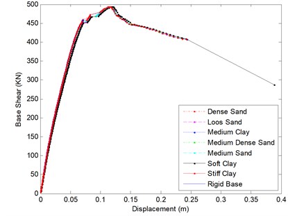
Fig. 12Pushover curve for 15 story frame – all soil types

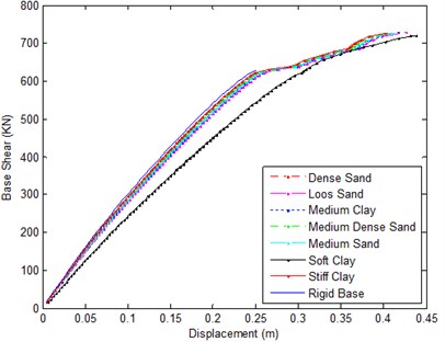
Fig. 13IDA curve for 3 story frame – all soil types

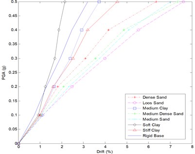
Fig. 14IDA curve for 6 story frame – all soil types

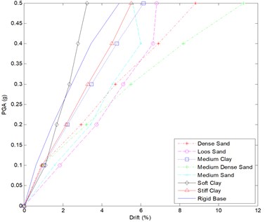
Fig. 15IDA curve for 9 story frame – all soil types

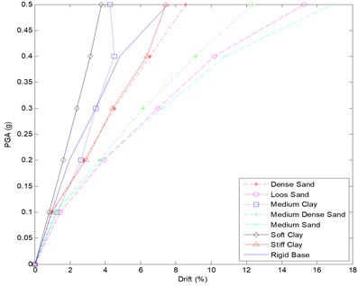
Fig. 16IDA curve for 12 story frame – all soil types

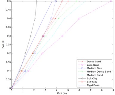
Fig. 17IDA curve for 15 story frame – all soil types

7. Evaluating average drift increase caused by SSI

7.1. Average drift increase for each frame on different soil types

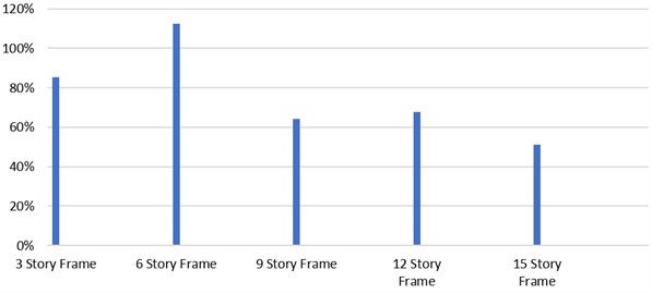
It is intended here to figure out the dependence of response augmentation, due to considering SSI, to the frame height and to find the response intensification trend in terms of the number of stories.

According to Table 13, the SSI effect on the average drift value is the most profound for the 6 story frame and the least powerful for the 15 story frame. Based on the resultant average values, it could be said that for low rise structures, as the structure becomes taller, the drift lengthening, as a result of considering SSI, swells. in addition, for medium rise structures, the frame height is not a governing parameter capable of either softening or magnifying the effect of SSI. for high rise structures, the effect of SSI on the drift wears off with increasing structural height. It should be noted that this fact was argued in a different manner in part 3.1.

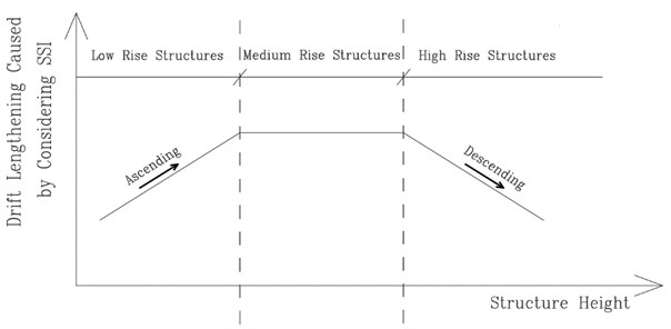
The most decisive effect of SSI on the drift belongs to the low and medium rise structures. a schematic graph representing the relation between “height of structures” and “drift lengthening caused by SSI” is demonstrated in Fig. 19.

Fig. 18Average of drift lengthening caused by considering SSI

Based on Fig. 19, it can be stated that, in the case of low rise structures, drift lengthening grows with increasing height of the structure, and for medium rise structures, the frame height doesn’t affect the drift lengthening; finally, for tall buildings, considering the SSI leads to a decline in drift lengthening. It is obvious that the most dramatic effect of SSI is produced for medium rise structures. in the case of very tall buildings, drift lengthening caused by SSI approaches zero, meaning that, for such buildings, considering SSI doesn’t affect the drift of the structure.

Table 13Drift increment due to considering SSI – classified based on story number

			Drift Increment (%)						Average drift increment due to SSI	Maximum drift increment due to SSI	Average for each frame
			PGA (g)
			0	0.1	0.2	0.3	0.4	0.5
3 story frame	Subsoil	Loose sand	0	50 %	91 %	107 %	124 %	139 %	85 %	139 %	85 %
		Medium sand	0	54 %	81 %	94 %	106 %	120 %	76 %	120 %
		Medium dense sand	0	41 %	61 %	84 %	97 %	130 %	69 %	130 %
		Dense sand	0	32 %	41 %	60 %	68 %	99 %	50 %	99 %
		Soft clay	0	23 %	–3 %	–13 %	–24 %	–33 %	–8 %	23 %
		Medium clay	0	43 %	28 %	24 %	18 %	17 %	22 %	43 %
		Stiff clay	0	35 %	24 %	31 %	29 %	43 %	27 %	43 %
6 story frame	Subsoil	Loose sand	0	200 %	154 %	108 %	92 %	39 %	99 %	200 %	112 %
		Medium sand	0	153 %	133 %	86 %	74 %	14 %	77 %	153 %
		Medium dense sand	0	54 %	120 %	124 %	137 %	131 %	94 %	137 %
		Dense sand	0	46 %	100 %	92 %	100 %	80 %	70 %	100 %
		Soft clay	0	80 %	15 %	–5 %	–20 %	–34 %	6 %	80 %
		Medium clay	0	64 %	53 %	42 %	38 %	26 %	37 %	64 %
		Stiff clay	0	53 %	48 %	34 %	31 %	13 %	30 %	53 %
9 story frame	Subsoil	Loose sand	0	49 %	100 %	101 %	111 %	102 %	77 %	111 %	64 %
		Medium sand	0	26 %	96 %	108 %	124 %	123 %	79 %	124 %
		Medium dense sand	0	18 %	87 %	77 %	89 %	64 %	56 %	89 %
		Dense sand	0	2 %	42 %	30 %	35 %	13 %	20 %	42 %
		Soft clay	0	–16 %	–17 %	–31 %	–34 %	–50 %	–25 %	0 %
		Medium clay	0	31 %	33 %	0 %	–6 %	–43 %	3 %	33 %
		Stiff clay	0	0 %	48 %	27 %	32 %	–2 %	18 %	48 %
12 story frame	Subsoil	Loose sand	0	125 %	101 %	116 %	113 %	143 %	100 %	143 %	68 %
		Medium sand	0	106 %	70 %	74 %	66 %	81 %	66 %	106 %
		Medium dense sand	0	40 %	39 %	46 %	48 %	60 %	39 %	60 %
		Dense sand	0	29 %	35 %	36 %	38 %	39 %	30 %	39 %
		Soft clay	0	10 %	–9 %	–19 %	–26 %	–38 %	–14 %	10 %
		Medium clay	0	76 %	49 %	35 %	25 %	8 %	32 %	76 %
		Stiff clay	0	40 %	38 %	33 %	31 %	24 %	28 %	40 %
15 story frame	Subsoil	Loose sand	0	77 %	37 %	32 %	23 %	20 %	31 %	77 %	51 %
		Medium sand	0	64 %	6 %	9 %	–1 %	16 %	16 %	64 %
		Medium dense sand	0	44 %	14 %	–3 %	–12 %	–41 %	0 %	44 %
		Dense sand	0	35 %	10 %	–7 %	–15 %	–45 %	–4 %	35 %
		Soft clay	0	45 %	38 %	26 %	23 %	0 %	22 %	45 %
		Medium clay	0	62 %	12 %	8 %	–3 %	0 %	13 %	62 %
		Stiff clay	0	31 %	–2 %	–1 %	–7 %	1 %	4 %	31 %

Fig. 19Schematic graph for relation between “height of structure” and “drift lengthening caused by SSI”

7.2. Average drift growth for different frames on the same soil type

In this part, the dependence of the average of response growth, due to considering SSI, on soil type is examined.

Table 14Drift increment due to considering SSI – classified based on soil type

		Drift increment (%)						Average drift increment due to SSI	Maximum drift increment due to SSI	Average for each frame
		PGA (g)
Subsoil	Story \PGA	0	0.1	0.2	0.3	0.4	0.5
Loose sand	3 Story	0	50 %	91 %	107 %	124 %	139 %	85 %	139 %	134 %
	6 Story	0 %	200 %	154 %	108 %	92 %	39 %	99 %	200 %
	9 Story	0 %	49 %	100 %	101 %	111 %	102 %	77 %	111 %
	12 Story	0 %	125 %	101 %	116 %	113 %	143 %	100 %	143 %
	15 Story	0 %	77 %	37 %	32 %	23 %	20 %	31 %	77 %
Medium sand	3 Story	0 %	54 %	81 %	94 %	106 %	120 %	76 %	120 %	113 %
	6 Story	0 %	153 %	133 %	86 %	74 %	14 %	77 %	153 %
	9 Story	0 %	26 %	96 %	108 %	124 %	123 %	79 %	124 %
	12 Story	0 %	106 %	70 %	74 %	66 %	81 %	66 %	106 %
	15 Story	0 %	64 %	6 %	9 %	–1 %	16 %	16 %	64 %
Medium dense sand	3 Story	0 %	41 %	61 %	84 %	97 %	130 %	69 %	130 %	92 %
	6 Story	0 %	54 %	120 %	124 %	137 %	131 %	94 %	137 %
	9 Story	0 %	18 %	87 %	77 %	89 %	64 %	56 %	89 %
	12 Story	0 %	40 %	39 %	46 %	48 %	60 %	39 %	60 %
	15 Story	0 %	44 %	14 %	–3 %	–12 %	–41 %	0 %	44 %
Dense sand	3 Story	0 %	32 %	41 %	60 %	68 %	99 %	50 %	99 %	63 %
	6 Story	0 %	46 %	100 %	92 %	100 %	80 %	70 %	100 %
	9 Story	0 %	2 %	42 %	30 %	35 %	13 %	20 %	42 %
	12 Story	0 %	29 %	35 %	36 %	38 %	39 %	30 %	39 %
	15 Story	0 %	35 %	10 %	–7 %	–15 %	–45 %	–4 %	35 %
Soft clay	3 Story	0 %	23 %	–3 %	–13 %	–24 %	–33 %	–8 %	23 %	32 %
	6 Story	0 %	80 %	15 %	–5 %	–20 %	–34 %	6 %	80 %
	9 Story	0 %	–16 %	–17 %	–31 %	–34 %	–50 %	–25 %	0 %
	12 Story	0 %	10 %	–9 %	–19 %	–26 %	–38 %	–14 %	10 %
	15 Story	0 %	45 %	38 %	26 %	23 %	0 %	22 %	45 %
Medium clay	3 Story	0 %	43 %	28 %	24 %	18 %	17 %	22 %	43 %	56 %
	6 Story	0 %	64 %	53 %	42 %	38 %	26 %	37 %	64 %
	9 Story	0 %	31 %	33 %	0 %	–6 %	–43 %	3 %	33 %
	12 Story	0 %	76 %	49 %	35 %	25 %	8 %	32 %	76 %
	15 Story	0 %	62 %	12 %	8 %	–3 %	0 %	13 %	62 %
Stiff clay	3 Story	0 %	35 %	24 %	31 %	29 %	43 %	27 %	43 %	43 %
	6 Story	0 %	53 %	48 %	34 %	31 %	13 %	30 %	53 %
	9 Story	0 %	0 %	48 %	27 %	32 %	–2 %	18 %	48 %
	12 Story	0 %	40 %	38 %	33 %	31 %	24 %	28 %	40 %
	15 Story	0 %	31 %	–2 %	–1 %	–7 %	1 %	4 %	31 %

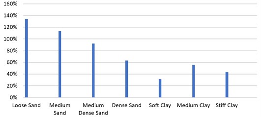
According to Table 14 and Fig. 20, it could be concluded from the average values that, for sandy soils, the SSI impact grows as the subsoil becomes looser, but for clay soils, medium clay produces the strongest SSI effect. the results obtained from Fig. 20 affirm that “sandy soils have a stronger effect on drift than clayey soils”. It is important to note that drift is proportional and related to internal forces of the structural members, but displacement isn’t proportional to the internal forces; therefore, usually both the drift and the displacement represent the structure behavior together, not independently.

Fig. 20Average of drift lengthening caused by considering SSI

8. Evaluating displacement gain due to SSI

Usually the main objective of analyses is finding internal forces and displacements. Internal forces are directly proportional to the drift, which was discussed in the previous section. in the present section, it is intended to study the effect of subsoil type on the structure displacements.

8.1. Base displacement

As mentioned earlier, earthquake input motion could vary from soil type to soil type. the foundation displacement for all subsoil types is discussed here.

Fig. 21Base displacement – 3 story

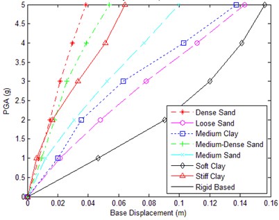
Fig. 22Base displacement – 6 story

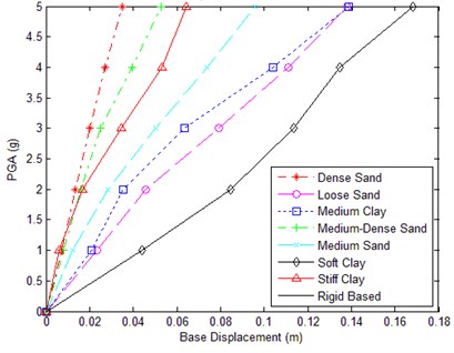
Fig. 23Base displacement – 9 story

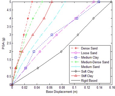
Fig. 24Base displacement – 12 story

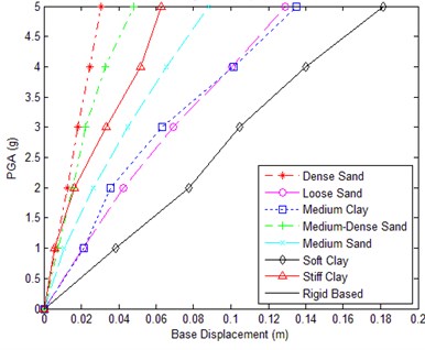
Fig. 25Base displacement – 15 story

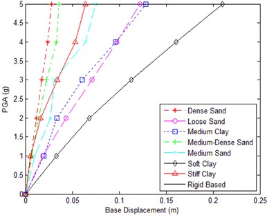
As it is obvious, input displacements depend highly on the subsoil types and partially on the structure height. It could be concluded from Figs. 21-25 that the looser the subsoil, the larger the foundation displacement under the action of earthquake. the presence of soft clay results in the highest base displacement values.

8.2. Roof displacement

In the previous section, the soil type effect on the input displacement was presented; the present section is aimed at examining the effect of soil type on roof displacement as the response of frames under the action of earthquake.

Fig. 26Roof displacement – 3 story

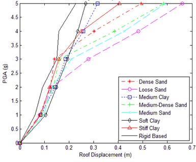
Fig. 27Roof displacement – 6 story

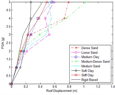
In the case of sandy soils, the largest roof displacement value generally belongs to the frames on the loose sand, and the roof displacement decreases for denser soils. the 3, 6 and 9 story frames on the soft clay have low values of roof displacement, even sometimes less than the rigid based frame, while such frames on the stiff clay produce higher roof displacement values. the frames on the soft clay behave somehow like an isolated structure which produces large base displacements but small inter-story displacements. the 15 story frame on the soft clay is characterized by having a greater roof displacement than the same frame on stiff clay. Simultaneous assessment of roof and base displacements reveals the fact that low and medium rise structures on soft clay behave like a rigid structure with large foundation displacements and low inter-story displacement values. Generally speaking, the largest value of roof displacement belongs to the frames located on loose and medium sand.

Fig. 28Roof displacement – 9 story

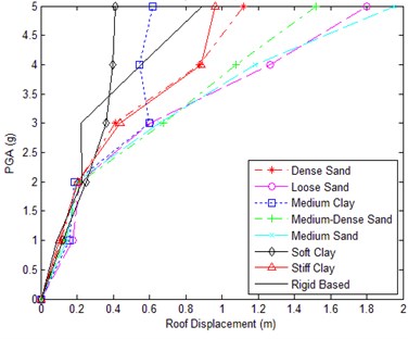
Fig. 29Roof displacement – 12 story

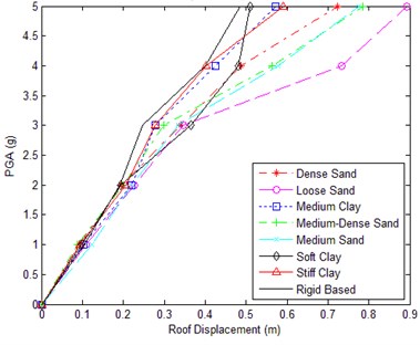
Fig. 30Roof displacement – 15 story

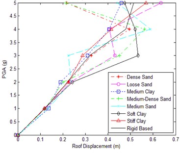
9. Conclusions

Seven soil types and five frames are considered in order to investigate the seismic behavior of various soil-structure systems. the innovative idea explored in the present paper is to consider a wide range of soil types and structure heights for examining the structural response trend under the effect of the changes in soil type and structure height. the base and roof displacements and the pushover and IDA curves of each soil-structure system are derived and evaluated. a comparison was made between the responses of the soil in the time and frequency domains. Based on all the aforementioned analyses, the following results are obtained:

1) In the case of sandy soils, the drift intensifies more considerably for looser soils. on the other hand, in the case of clayey sub-soils, for 3 to 12 story frames, the stiff clay causes the most profound drift lengthening, and the soft clay produces the weakest drift lengthening; but with the 15 story frame, the opposite is the case (According to Figs. 13-17).

2) Based on the average values, the effect of SSI on the drift is the strongest for the 6 story frame and is the least powerful for the 15 story frame.

3) Generally speaking, it could be said that for low rise structures, the drift lengthening, caused by SSI, grows with increasing structure height, and for medium rise structures the frame height is not a governing parameter on the SSI effect; lastly for high rise structures, “the taller the structure, the less profound the effect of SSI on the drift” (According to Table 11).

4) The soft clay is the only soil which causes the drift values to be lower than those of fixed-based structures for 3 to 12 story frames, but this soil induces the most considerable drift lengthening for the 15 story frame. This phenomenon can be interpreted by the fact that “soft soil deposits amplify low frequency components of earthquake and attenuate high frequency ones, while just the opposite applies for stiff soils; therefore, high rise frames with low natural frequency values would resonate on soft deposits and vice versa” (Based on Figs. 13-17).

5) Generally, stiff soils amplify the responses of low rise structures and may reduce those of high rise structures; the opposite applies for soft soils.

6) The drift of the structure on the soft soil doesn’t increase a lot with increasing PGA, confirming that, in the case of soft soils, for high PGA’s the soil enters the nonlinear state and doesn’t allow the structure to suffer from higher amounts of drift. Such a phenomenon is somewhat similar to the behavior of isolated structures (According to Figs. 13-17).

7) It could be concluded that for taller structures (lower natural frequencies), loose sub-soils alter the responses more significantly than stiff soils, but in the case of short structures (high natural frequency), stiff sub-soils change the responses more substantially than soft soils.

8) Earthquake input displacement (foundation displacement) depends greatly on the subsoil type and partially on frame height. Soft soils induce larger displacements in the foundation (Based on Figs. 21-25).

9) For sandy soils, the looser the subsoil, the larger the roof displacement for all frames.

10) Low and medium rise structures on soft clay exhibit a rigid structural behavior with large foundation displacements and small inter-story displacements; therefore, the roof displacements of low and medium rise frames on the soft clay could even be smaller than those of the rigid base frames (According to Figs. 21-25).