Abstract
The concept of inertia coupling terms among substructures was proposed. Based on the branch mode method, the superstructures and foundation soil of one soil-adjacent structure system were divided into different branches. The branch mode method was effectively introduced to real-time dynamic substructure testing (RTDST) by decomposing and transforming the motion equation of the entire system. It was also applied for the interaction coupling terms to exchange data between the physical and numerical substructures. This method decreased the degree-of-freedom of the linear substructure effectively and considered the effects of foundation translation and rotation on the upper structures. One system composed of two adjacent four-story steel structures (S1 and S2, respectively) and foundation soil was presented in this study. S1 was applied on a shaking table as the physical substructure, whereas the foundation soil and S2 were set as two numerical substructures and simulated in a computer. The seismic response of the entire coupling system was analyzed by real-time data exchange among substructures. Test results agree with numerical solutions. The RTDST based on the branch mode method is a feasible and reliable method for the investigation of soil-adjacent structure interaction (SASI) problems, and provides a new way to consider SASI problems in the RTDST.
1. Introduction
Given the advancement of means and methods to study the soil-structure interaction (SSI) problems [1, 2], the problem of soil-adjacent structure interaction (SASI) [3-6] attracts more attention from researchers in recent years. Theoretical analysis methods of SSI mainly include overall and substructure analyses. In the experimental studies, indoor model testing and prototype measurement are often used to solve SSI problems, which can also be introduced to the SASI problem. Researchers have achieved a series of valuable theoretical conclusions and outcomes after unceasing endeavors [6]; however, they gained few achievements in an experimental study because of the complexity and size of the adjacent structure system, as well as the limitations under laboratory conditions. Aldaikh H. et al. carried out a shake table test of the dynamic interaction on a group of three buildings. The adverse and beneficial effects of SASI under seismic excitation were explored [7].
At present, the shaking table test is an effective method for a structural model test. The model soil box method [8-10] is common in a shaking table test that considers SSI. The method starts with fixing a predesigned and full-model soil box at a shaking table. The superstructure model is subsequently placed above soil mass. Then, the ground motions of an earthquake are applied through the shaking table to accomplish the test. However, the model soil box method still has various limitations. Test results are bound to be affected by the restricted bearing capacity of the shaking table and the manual model boundary conditions of the soil box. The limited space allotted for foundation soils cannot fully simulate the scattering of seismic waves.
The real-time dynamic substructure testing (RTDST) [11-13] provides a new method for solving SSI and SASI problems. This method is currently an important development trend for testing the earthquake resistance of a large complicated structure system. Researchers started the procedure by dividing the building structure into several substructures. They used the bottom [14], middle [17], or top substructures [18] as a physical substructure, and uploaded it using an actuator [14-16] or shaking table [18-20], or both [17]. The remaining substructures were used as numerical substructures and simulated in a computer through the established numerical models. The dynamic response of the entire structure was analyzed through real-time coupling. The RTDST was applied to a two-story steel frame structure in Reference [21], considering SSI by setting the foundation soil as the numerical substructure. The foundation soil was simplified as two degrees of freedom unduly and the acceleration impact of foundation rotation was not considered for the superstructure. In previous tests, the interfacial force for data exchange between physical and numerical substructures worked as the horizontal shear force. In engineering practice, experimental studies of SSI or SASI problems produce excellent results when the impacts of foundation translation and rotation on the superstructure are considered. However, the RTDST of SSI and SASI has two challenges. First, if the foundation soil is set as a physical substructure, then only the foundation soil within a limited range can be simulated. This limitation is due to the restricted bearing capacity and size of the shaking table, which only allows the superstructure model to occupy a considerably small portion of the test structure. These factors significantly influence test results [22]. Second, if the foundation soil is set as a numerical substructure, then it is calculated in real-time and the data exchange becomes challenging. This difficulty is due to a large amount of DOFs of the foundation soil, and the fact that the loading step of RTDST finishes in a few milliseconds. Narrowing of the computation scale of the numerical substructure to increase the computation efficiency and convenient solution of the problem to RTDST after reasonable simplification are important issues to be resolved.
The branch mode method [23]is a dynamic substructure method that can significantly reduce the DOFs of structures and computation scale. This method is used for a dynamic analysis and solution of linear structures. In this study, the branch mode method was introduced into the RTDST of SASI. On the basis of this method, the concept of the coupling term was used in data exchange and transmission between physical and numerical substructures, in order to provide convenient conditions to study the SASI in RTDST. The branch mode method divided the superstructures and foundation soil in the soil-adjacent structural system into different substructures. This method could be used in the RTDST effectively with inertial coupling terms among different substructures by decomposing and transforming the kinetic equation of the entire system. In this study, an RTDST based on a shaking table considering SASI was implemented to the soil-adjacent structure system, which was composed of two same-steel structures and foundation soil. Each steel structure has four stories and one span. The SASI mechanism and law were explored by analyzing test results under different working conditions, which fully reflected the RTDST characteristics based on the branch mode method. Results provided data support and experimental verification for studying such a complicated system and related problems.
2. Theory of branch mode method and its application in RTDST
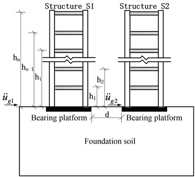
For the effective use of the branch mode method for the RTDST of SASI, the soil-adjacent structure system in Fig. 1 is divided into three substructures: foundation soil substructure D, and upper substructures S1 and S2. These substructures are analyzed in this section, respectively.
2.1. Substructure D analysis
The research indicated that only a small region of the foundation soil, which was remarkably close to the upper structures, would produce plastic strain when the texture of the foundation soil was good in a seismic response analysis. Conversely, the foundation soil region, which is far from the upper structures, has the linear working condition throughout the process of seismic excitation. Thus, the entire structure system may have local nonlinear characteristics under earthquakes. For convenience, foundation soil is simplified to be elastic in this study. For the linear foundation soil substructure, stiffness , mass , and damping matrices of the elastic foundation are used to obtain the eigenvalue problem:
where is a characteristic value, and is the dominant mode of substructure D. According to Eq. (1), the first orders of the dominant modes are obtained and then the modal matrix is formed as follows:
where ,,…, are the first orders of the dominant modes of foundation soil substructure. Characteristic matrices of D after the modal transformation are:
where , , , and are the generalized stiffness, mass, damping, and external load matrices, respectively, after the degrees of freedom (DOFs) of the linear foundation soil substructure have been reduced. can be calculated by the general damping theory, and load matrix is the earthquake input load at the bearing platform.
Fig. 1Soil-adjacent structure system
2.2. Substructure S1 (S2) analysis
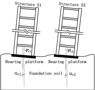
Given that S1 (S2) involves relatively few DOFs, the DOFs of S1 (S2) are not reduced to meet the elastic-plastic analysis. If the bearing platform is rigid, then the acceleration at different points of the bearing platform will be the same. The deformation pattern of the upper structures is shown in Fig. 2. Horizontal and angular displacements of the upper bearing platform surface at S1 (S2) caused by foundation deformation are marked as and ( and ), respectively (Fig. 3). The deformation (or displacement) of the foundation soil will cause the rigid body displacement of the upper structures; thus, the rigid mode of S1 can be calculated by the base point method (using the surface center of the bearing platform as the base point). The horizontal displacement of S1 at any height () is:
where is the distance from any height of S1 to the top foundation (Fig. 1). Subsequently, the rigid mode matrix of S1 () is obtained as follows:
where is a matrix, is the number of stories and is the number of DOFs of the foundation soil. Similarly, the rigid mode matrix of S2 () can be achieved.
Fig. 2Deformation pattern of upper structures (rigid foundation)
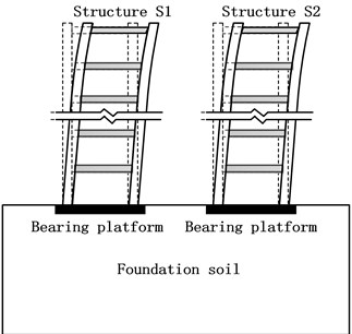
Fig. 3Rigid body displacement of upper structures caused by foundation deformation
2.3. Motion equation building
The implemented modal is substituted into transformation, considering and . The relationship between the physical and generalized coordinates of the substructures can be obtained as follows:
where , , and are displacement vectors of substructures D, S1, and S2, respectively, under the physical coordinates. , , and are displacement vectors of three substructures under the generalized coordinates. Based on Eq. (6), the entire equation of motion of S1 and S2 with physical coordinates, and the linear foundation substructure with the generalized coordinates is obtained as follows:
where , , , and are stiffness, mass, damping, and external load matrices of substructure D, respectively, with the generalized coordinates; , , , and are stiffness, mass, damping, and external load matrices of S1, respectively, with the physical coordinates; and , , , and are the related matrices of S2 with the same meanings as S1.
2.4. Equation of branch modal transformation and its application in RTDST
Eq. (7) is the dynamic equation of the soil-adjacent structure system. This equation reveals that the mass matrix has non-diagonal items (i.e., and ) that combine S1, S2, and D. Herein, the items are named as interaction coupling terms. For RTDST, the data exchange between physical and numerical substructures is completed through mutual transmission of interfacial force. Eq. (7) is divided into motion equations of D, S1, and S2 for the RTDST of soil-adjacent structure system, and unknown coupling items are moved to the right of equations, as follows:
where:
In Eqs. (11-12), is a unit matrix. and are ground accelerations applied onto the bearing platforms of S1 and S2, respectively; is the traveling wave of (Fig. 1), which only has time delay and amplitude attenuation. Two variables meet, as shown as follows:
where is the amplitude attenuation coefficient (); is the distance between two bearing platforms; and are the velocity and time of seismic wave propagation, respectively.
In Eqs. (8-10), the interaction coupling items appear as a load when they are on the right of the equations. The interaction coupling forces are obtained by multiplying the interaction coupling items with the related terms. The interaction coupling forces constitute the external forces of three substructures together with the earthquake forces on D, S1, and S2 (, , and ), respectively. The interaction coupling forces can be calculated given that acceleration vectors of S1 and S2 ( and , respectively) are known. The motion equation of the foundation soil (Eq. (8)) can be solved. The calculated acceleration vector of the foundation soil () is brought into Eqs. (9-10) to implement the independent loading of S1 and S2, respectively, thereby providing a great convenience to the shaking table-based RTDST.
3. Test design
3.1. Division of physical and numerical substructures
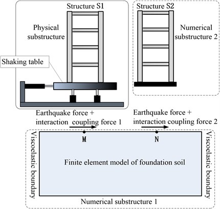
The transformed branch mode method can use the above interaction coupling terms in the loading of upper substructures and in the independent numerical solution of the foundation soil substructure; thus, this method is used in the RTDST of SASI in this study. The substructure division of the soil-adjacent structure system, composed of two similar four-story shear frames and foundation soil, is shown in Fig. 4. In the RTDST, physical substructures should be set according to equipment conditions and interested substructures. Foundation soil involves the bearing capacity and table size of the shaking table, as well as soil boundary settings. Thus, S1 is set as a physical substructure for a load test on the shaking table, whereas S2 and D are set as two numerical substructures. The seismic response of the entire system is analyzed through real-time data transmission among different substructures. In the test, the SIMULINK simulation program is applied for signal transmission and solution of the motion equation. Meanwhile, S2 is set as an independent numerical substructure to be prepared for the follow-up shaking tables test. The data exchange method between S2 and D is the same as that for S1.
Fig. 4Division of physical substructure and numerical substructure
3.2. Parameters and similarity relations of physical substructure
To make the model structure, the dynamic features of the prototype structure are reflected, and the test model is designed according to the similarity theory. In this test, 1:5 scale model is applied to the physical substructure. The main parameters and similarity relations of the model are listed in Table 1. The plane dimension of the physical substructure (Fig. 5) is 1.6 m×1.6 m. The height of the ground floor is 0.68 m, and that of the other floors is 0.63 m, with the total height of 2.57 m. All beams and columns use H-shaped Q345 steel.
Fig. 5Physical substructure
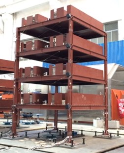
Table 1Main model parameters and similarity relations
Parameters | Expressions | Similarity relations | Parameters | Expressions | Similarity relations |
Modulus of elasticity | 1 | Mass | 0.04 | ||
Length | 0.2 | Stiffness | 0.2 | ||
Time | 0.45 | Acceleration | 1 |
The cross-section dimension is 100 mm×45 mm×6 mm×8 mm. Elasticity modulus 2.02×10⁵ MPa is measured in a material property test. Floors use 3-mm-thick steel plates, and one horizontal and one vertical beam are underneath the floors. Masses of different floors are 1.7×10³ kg, and 1.54×10³ kg. The resonant fixed-base period of structure S1 is 0.42 s, and the damping ratio is 0.02.
3.3. Numerical substructures
3.3.1. Adjacent structure (S2)
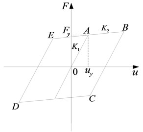
In the test, S2 is divided as an independent numerical substructure. S2 is simplified into a serial multi-DOF system, which is a shear model (Fig. 6). The mass of each story of the structure () is concentrated on the floor, and the stiffness of each story () is the sum of the lateral stiffness of all columns on this floor. Meanwhile, the double broken line constitutive model, known as the Ramberg-Osgood model, is used (Fig. 7). In Fig. 7, is the yield load, is yield displacement, is the initial shear stiffness, and is the post-yield stiffness (, where is the stiffness reduction coefficient and is 0.01 in this test). The masses of floors in S2 are the same with those in S1. The story stiffness of the ground floor is 3.87×10⁶ N/m, and story stiffness of the second to fourth floors is 4.86×10⁶ N/m.
Fig. 6Simplified model of S2
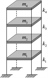
Fig. 7Double broken line constitutive model
3.3.2. Foundation model
In the SSI problem, the boundary effect slightly influences the dynamic response of the structure when free boundaries are applied to the sides of the foundation soil, and given that the plane size ratio between the foundation soil and structure is higher than five. In this study, the length, width, and depth of the foundation soil are set as 30 m, 15 m, and 15 m, respectively. The buried foundation sizes are 2.2 m×2.2 m×0.4 m. The material foundation parameters and the different soil mass layers are listed in Table 2. According to the consensus of the Rock Physical Simulation Technical Committee of International Association for Soil Mechanics and Geotechnical Engineering, the deformation trend of soil particles and the agglomeration effect of particle motion in the model are almost similar with those of an undisturbed soil when the model/soil particle size in the model is higher than 175 [24]. This soil mass can be used as model test materials. Therefore, the similarity of the foundation soil in this study is determined as one.
When soil mass is considered as a numerical substructure in the analysis, a three-dimensional finite element analysis model is used, where the bottom of the soil mass is fixed, and viscoelasticity boundaries are set surrounding the soil mass. The foundation soil is simplified appropriately considering the long computation time because of the abundant DOFs involved in a finite element model of the foundation, as well as the timeliness (generally 0-99 ms) of data transmission between the physical and foundation soil substructures. Given that the width direction of the foundation soil is not the main vibration direction, relative displacements of different nodes along the width direction are relatively small and viewed approximately consistent. On this basis, modal reduction of the foundation soil is conducted. Relative model parameters are listed in Table 3. The specific implementation method is introduced as follows.
Table 2Material parameters of foundation and foundation soil
Material type | Material No. | Thickness (m) | Elasticity modulus (Pa) | Density (kg/m3) | Poisson’s ratio |
Foundation | 1 | 0.4 | 3.5×10¹⁰ | 2650 | 0.2 |
Soil layer | 2 | 3.6 | 2.1×10⁸ | 1730 | 0.3 |
3 | 8.4 | 3.6×10⁸ | 1950 | 0.3 | |
4 | 3.0 | 4.3×10⁸ | 2030 | 0.3 |
1) The numerical substructure model of the foundation soil is established in the finite element software ANSYS. The mass, stiffness, and principal modal of the foundation soil substructure are extracted.
2) Data are inputted into MATLAB for an analysis. All calculated soil mass modals are rescreened and ranked in the descending order according to the mass participation coefficient along the vibration direction. The final computing modal number, together with the requirements on analysis accuracy and computation power of test equipment, is determined (Table 3) to make the sum of the mass participation coefficients of the vibration model reach the value higher than 95 %.
3) The chosen modal number is used in Eq. (3) to calculate the modal mass and the stiffness matrices of the soil mass. The modal damping matrix can be calculated according to the Rayleigh damping assumption. Subsequently, these three matrices are inputted for computation in the Simulink program of the soil-adjacent structure system based on the branch mode method. This treatment method reduces the order of the characteristic matrix of linear foundation soil substructure. Therefore, the goal of DOFs reduction and high-efficiency computation is achieved, guaranteeing real-time computation in the RTDST.
Table 3Parameters of finite element model of foundation soil
Length (m) | Width (m) | Depth (m) | Element type | Element size (m) | Element number | Node number | Number of DOFs | Number of chosen mode |
30 | 15 | 15 | Solid45 | 1 | 15876 | 17974 | 2286 | 60 |
3.4. Test
In this test (Fig. 3), the overall model is divided into a physical substructure S1 and two numerical substructures (foundation soil and upper substructure S2) based on the branch mode method. The dynamic interactions of these substructures are achieved by the force balance and displacement coordination at the connection points. The experiment was conducted on the shaking table. The main parameters and technical indexes of the shaking table are as follows. The table sizes of the shaking table are 3 m×3 m; the platform weight is 60 kN; the maximum weight of the specimens is 100 kN; the frequency range is 0.1-50 Hz; the shaking table only shakes in the horizontal direction; and the control method is used with three-parameters simulation and digital iteration.
Eq. (4) and Eq. (9) show that the seismic excitation to S1 is composed of the horizontal earthquake acceleration , as well as the translation () and rotation () accelerations of the foundation that causes rigid body displacement of the upper substructures. In the RTDST based on the branch mode method, and , but not , can be applied to S1 through the shaking table. The effect of on S1 is the horizontal inertial load related to the height; thus, the horizontal inertia force in an inverted-triangle distribution caused by at the lumped mass of S1 is equivalent to an evenly distributed horizontal inertia force. This finding follows the principle of base shear force equivalence (unrelated to the height after equivalence, and the equivalence coefficient is 1.6).
In the test, the acceleration vector of S1, which is measured by the sensor (), the calculated acceleration vector of S2 (), and seismic force (Eq. (8)), are inputted into the numerical foundation soil substructure for the implementation using the Simulink program. The calculated acceleration vector of the foundation soil () is used in Eqs. (9-10), and the interaction coupling force is gained. The physical substructure S1 and numerical substructure S2 are uploaded and solved after the superposition of the interaction coupling force and seismic force.
Fig. 8Test flowchart
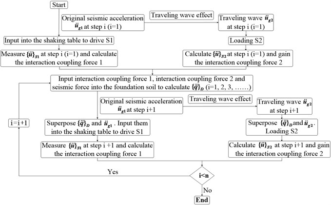
The entire process of test is divided into equal steps:
1) The original seismic acceleration record at step is inputted into the physical substructure S1 through the shaking table. Meanwhile, , which is gained at step after the traveling wave effect, is applied to the numerical substructure S2. The acceleration () of the physical substructure S1 at step , which is used to calculate the interaction coupling force 1 (Eq. (8)), is measured. Simultaneously, the acceleration () of the numerical substructure S2 at step , when the traveling wave effect is considered, is calculated and used to compute the interaction coupling force 2 (Eq. (8)).
2) The interaction coupling forces 1 and 2, and the seismic forces (Eq. (8)) are inputted into the foundation soil substructure as external forces for a numerical calculation. Subsequently, the acceleration vector () of the foundation soil at step can be calculated.
3) The superposition of at step and the original seismic acceleration () at step () is inputted into S1 through the shaking table. Meanwhile, the superposition of and is inputted into the numerical substructure S2. , which is used to calculate the interaction coupling force 1, is measured. Simultaneously, is calculated and used to derive the interaction coupling force 2.
4) Steps (2) and (3) are repeated until the end of test.
In this process, each loading time step is accomplished timely, thus obtaining real dynamic response of the entire structural system to a given earthquake force. The test flowchart is shown in Fig. 8.
In the test, the collected data of S1 is inputted into the numerical substructure of the foundation soil in a control computer through an I/O equipment plate. The seismic response data of S2 is transmitted simultaneously to the numerical substructure of the foundation soil by combining Newmark- method and Newton-Raphson iteration. The numerical substructure of the foundation soil is solved using the state-space equation method [25]. Calculated data is used as the output command and output to the control system of the shaking table through the I/O equipment plate to drive S1. The remaining data is directly transmitted to S2. This way, a closed circulation pathway for the real-time data exchange is established among three substructures through the data acquisition system, I/O equipment plate, and Simulink simulation platform in the control computer. The Simulink simulation platform comprises the main program of state-space equation of the foundation soil, the elastic-plastic analysis subprogram of S2, and analog input and output. All of these forms the RTDST for soil-adjacent structure system based on the branch mode method.
4. Test result analysis
4.1. Seismic motion input
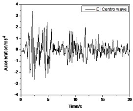
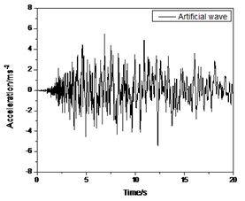
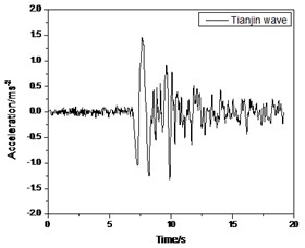
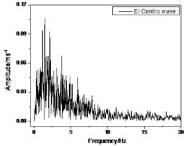
In this study, El Centro, artificial, and Tianjin waves are used as seismic motion inputs of the test. The time history and corresponding Fourier spectrum are presented in Figs. 9-10, respectively. S1, S2, and soil mass are in the elastic state under the effect of frequently occurring earthquakes according to the numerical simulation analysis before the test. However, the soil mass is still under the elastic state under moderate and rarely expected earthquakes, whereas S1 and S2 enter into a nonlinear working state. In the test, the amplitudes of three seismic waves are regulated. Frequently occurring (0.07 g), moderate (0.2 g), and rarely expected (0.3 g) earthquakes are loaded, respectively.
Fig. 9Time history of earthquake waves used in RTDST
a)
b)
c)
Fig. 10Fourier spectrum of earthquake waves used in RTDST
a)
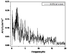
b)
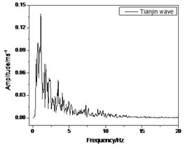
c)
4.2. Analysis of test results
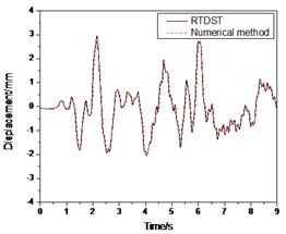
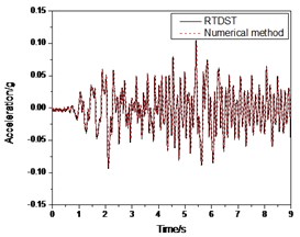
To verify the accuracy and validity of RTDST based on the branch mode method, a numerical simulation of the soil-adjacent structure system is performed using the branch mode substructure method. Calculated results of the numerical simulation method are compared with RTDST results. S2 and foundation soil in the numerical simulation are equivalent with those in the RTDST. S1 is simplified into a serial multi-DOF system, which is a shear model. Eq. (8) is solved by the Newmark- method. Comparisons between RTDST and numerical simulation results of S1 under the El Centro wave (0.07 g, 0.2 g), Artificial wave (0.07 g, 0.2 g) and Tianjin wave (0.07 g, 0.2 g, and, 0.3 g) are presented in Figs. 11-17, respectively.
Fig. 11Seismic response of S1 under El Centro wave (0.07 g)
a) Displacement time-history of top floor center
b) Acceleration time-history of top floor center
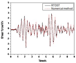
c) Shear force time-history of ground floor
Fig. 12Seismic response of S1 under El Centro wave (0.2 g)
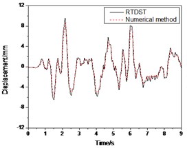
a) Displacement time-history of top floor center
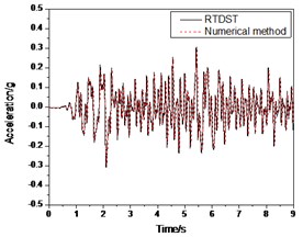
b) Acceleration time-history of top floor center
c) Shear force time-history of ground floor
Figs. 11-12 show the comparison between the results of RTDST and numerical simulation under the El Centro wave (0.07 g and 0.2 g, respectively). They are consistent with each other with regard to amplitudes and frequencies.
In Fig. 11, the peaks of the top floor displacement, acceleration and ground floor shear force are 2.96 mm, 0.104 g and 3.78 KN, respectively, by the RTDST while the numerical simulation results are 2.83 mm, 0.101 g and 3.57 KN, correspondingly. The errors are 4.7 %, 2.9 % and 5.8 %, respectively.
From Fig. 12, in the peak comparison, the numerical solutions of top floor displacement and acceleration are 8.74 mm and 0.294 g, respectively, while the RTDST results are 9.56 mm and 0.309 g. Thus, the errors are 9.4 % and 5.1 %, respectively. For ground floor shear force, the numerical solution is 11.08 KN while the experimental result is 11.23 KN, or an error is 1.4 %.
Figs. 13-14 show the comparison between the experimental and numerical results under the Artificial wave (0.07 g and 0.2 g, respectively) and they produced almost identical results except that there are some differences in amplitude between two time histories.
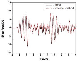
In Fig. 13, the numerical results of the top floor displacement peak, top floor acceleration peak and maximum shear force of the bottom story are 8.335 mm, 0.150 g and 4.78 KN, respectively, while the test results are 9.44 mm, 0.15 5 g and 5.25 KN with errors of 13.2 %, 3.2 % and 9.6 %, respectively.
In Fig. 14, the amplitudes of the test results are bigger than those of the numerical solution. For the displacement peak comparison, the experimental result is 26.85 mm while the numerical solution is 25.98 mm. The error is 3.3 %. The peak of the top floor acceleration in test is 0.418 g with an error of 2.7 % in comparison to the numerical simulation. For the ground floor shear force, the peak is 14.21 KN while the numerical result is 13.58 KN, or an error is 4.6 %.
Fig. 13Seismic response of S1 under Artificial wave (0.07 g)
a) Displacement time-history of top floor center
b) Acceleration time-history of top floor center
c) Shear force time-history of ground floor
Fig. 14Seismic response of S1 under Artificial wave (0.2 g)
a) Displacement time-history of top floor center
b) Acceleration time-history of top floor center

c) Shear force time-history of ground floor
Fig. 15Seismic response of S1 under Tianjin wave (0.07 g)
a) Displacement time-history of top floor center
b) Acceleration time-history of top floor center
c) Shear force time-history of ground floor
The comparison of RTDST and numerical simulation results under the Tianjin wave (0.07 g) is shown in Fig. 15. The maximum displacement of the top floor center, acceleration peak of the top floor center, and the maximum shear force of the ground floor are 9.16 mm, 0.227 g, and 11.85 KN in RTDST but 8.54 mm, 0.205 g, and 10.41 KN, in the numerical simulation, showing differences of 7.3 %, 10.7 %, and 13.8 %, respectively.
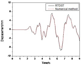
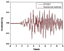
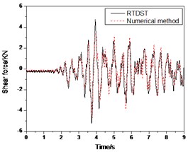
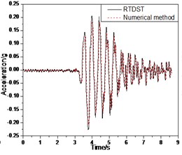
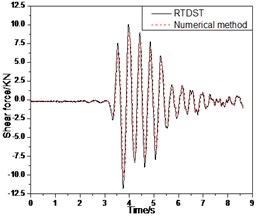
Fig. 16 shows the comparison between the results of RTDST and numerical simulation under the Tianjin wave (0.2 g). The maximum displacement of the top floor center, the acceleration peak of the top floor center, and the maximum shear force of the ground floor are 26.14 mm, 0.528 g, and 27.75 KN in the RTDST respectively. However, in the numerical simulation, the results are 24.91 mm, 0.497 g, and 25.58 KN, showing differences of 4.9 %, 6.2 %, and 8.5 %, respectively, in comparison with the RTDST.
Fig. 16Seismic response of S1 under Tianjin wave (0.2 g)
a) Displacement time-history of top floor center
b) Acceleration time-history of top floor center
c) Shear force time-history of ground floor
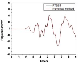
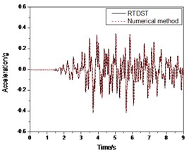
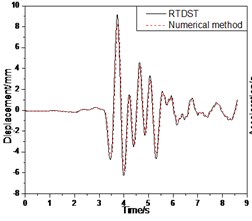
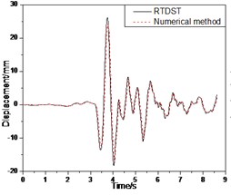
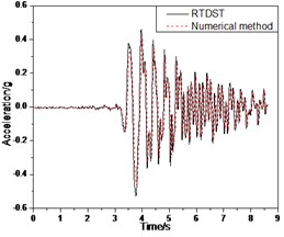
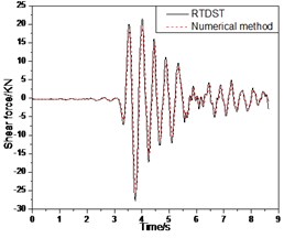
Fig. 17Seismic response of S1 under Tianjin wave (0.3 g)
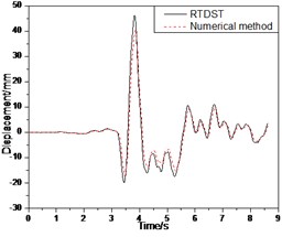
a) Displacement time-history of top floor center
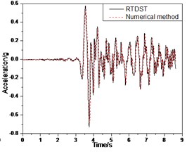
b) Acceleration time-history of top floor center
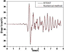
c) Shear force time-history of ground floor
The comparison of the results of RTDST and numerical simulation under the Tianjin wave (0.3 g) is shown in Fig. 17. The maximum displacement of the top floor center, acceleration peak of the top floor center, and the maximum shear force of the ground floor are 46.13 mm, 0.732 g, and 36.49 KN in the RTDST but 40.35 mm, 0.679 g, and 33.41 KN in the numerical simulation, with differences of 14.3 %, 7.8 %, and 9.3 %, respectively.
From the comparisons between test results and numerical solutions, it can be found that they coincide well with each other in regard to vibration frequency despite existing some differences in vibration amplitude. The RTDST based on the branch mode method can obtain satisfactory results. The accuracy is acceptable even though some errors still occur in test. The errors are mainly attributed to two aspects. First, the controlling accuracy of the shaking table, the measurement accuracy of the experimental instrument, and noise of the electronic equipment have influenced the test results. Second, the serial multi-DOF system shear model, which is a simplification of S1 in numerical simulation, is bound to cause errors.
In the test, the presented case is simple, but the problem will become very complicated after considering the numerical experimentation of foundation soil substructure. On one hand, with the increase of the DOFs of numerical substructure, it will be more difficult in a real-time computation and data exchange because the loading step in the RTDST must be finished in a few milliseconds. On the other hand, the controlling accuracy and stability of the shaking table is a great challenge for a large-scale physical substructure with a heavy weight. The agreement between test results and numerical solutions proved the correctness of the proposed method. In addition, the application of substructure equations to RTDST is another key problem not solvable so easily. In the process of implementation, inertia coupling terms in substructure equations are used to obtain interaction coupling forces on the interface of the foundation and superstructures. For the shaking table that can only vibrate in the horizontal direction, it also involves the equivalence and transformation of the foundation wobble effect here. Both the real-time data exchange between substructures and loading of the upper substructures precisely benefit from the reliability of the substructure equations.
5. Conclusions
The branch mode method is introduced into the RTDST of soil-adjacent structure system in this study. A soil-adjacent structure system composed of two adjacent steel structures and foundation soil is built. One steel frame is set as the physical substructure, and the rest ones are set as the numerical substructures for the RTDST based on a shaking table, which considers the SASI effect. The method is a novel way to study SASI problems. The research scope is expanded to the structure seismic test. The main conclusions are summarized as follows.
1) The upper structures and foundation soil of the soil-adjacent structure system are divided into different substructures based on the branch mode method. The concept of coupling item is proposed and used in the data exchange between physical and numerical substructures. The branch mode method is applied into the RTDST effectively.
2) Given that rotation acceleration produced by foundation deformation in test cannot be applied to the experimental substructure through the shaking table, it is converted into an equivalent horizontal acceleration according to the principle of base shear equivalence. This equivalent horizontal acceleration can be conveniently applied to the experimental substructure through the shaking table, further increasing the accuracy of RTDST.
3) The calculation efficiency of the numerical substructure of the foundation soil increases significantly through reasonable effective reduction of the DOFs of the foundation soil substructure. This solution guarantees the real-time calculation and data exchange. The solution also has a certain reference to the RTDST of complicated structure system with abundant DOFs and large computation scale.
4) The comparative analysis between RTDST and numerical simulation results verifies that the proposed RTDST based on the branch mode method is a feasible and reliable method to study SASI problems, which provides a novel idea and method to the RTDST of SSI or SASI.
References
-
Jiang X. L., Kuang Y. P., Jiang N. Inelastic parametric analysis of frequencies and seismic responses of soil-multistorey bidirectional eccentric structure interaction system. Journal of Vibroengineering, Vol. 18, Issue 5, 2016, p. 3010-3036.
-
Guo J., Tang Z. Y., Chen S. C., Li Z. B. Control strategy for the substructuring testing systems to simulate soil-structure interaction. Smart Structures and Systems, Vol. 18, Issue 6, 2016, p. 1169-1188.
-
Ghergu M., Ionescu I. R. Structure-soil-structure coupling in seismic excitation and “city effect”. International Journal of Engineering Science, Vol. 47, Issue 3, 2009, p. 342-354.
-
Ghandil M., Behnamfar F., Vafaeian M. Dynamic responses of structure-soil-structure systems with an extension of the equivalent linear soil modeling. Soil Dynamics and Earthquake Engineering, Vol. 80, 2016, p. 149-162.
-
Ghandil M., Aldaikh H. Damage-based seismic planar pounding analysis of adjacent symmetric buildings considering inelastic structure-soil-structure interaction. Earthquake Engineering and Structural Dynamics, Vol. 46, Issue 7, 2017, p. 1141-1159.
-
Lou M. L., Wang H. F., Chen X., Zhai Y. M. Structure-soil-Structure interaction: Literature review. Soil Dynamics and Earthquake Engineering, Vol. 31, Issue 12, 2011, p. 1724-1731.
-
Aldaikh H., Alexander N. A., Ibraim E., Knappett J. Shake table testing of the dynamic interaction between two and three adjacent buildings (SSSI). Soil Dynamics and Earthquake Engineering, Vol. 89, 2016, p. 219-232.
-
Pitilakis D., Dietz M., Wood W. D., Clouteau D., Modaressi A. Numerical simulation of dynamic soil–structure interaction in shaking table testing. Soil Dynamics and Earthquake Engineering, Vol. 28, Issue 6, 2008, p. 453-67.
-
Turan A., Hinchberger S. D., El Naggar M. H. Seismic soil-structure interaction in buildings on stiff clay with embedded basement stories. Canadian Geotechnical, Vol. 50, Issue 8, 2013, p. 858-873.
-
Lemnitzer A., Keykhosropour L., Kawamata Y., Towhata I. Dynamic response of underground structures in sand: experimental data. Earthquake Spectra, Vol. 33, Issue 1, 2017, p. 347-372.
-
Nakata N., Stehman M. Compensation techniques for experimental errors in real-time hybrid simulation using shake tables. Smart Structures and Systems, Vol. 14, Issue 6, 2014, p. 1055-1079.
-
Zhang Z. L., Staino A., Basu B., Nielsen S. R. K. Performance evaluation of full-scale tuned liquid dampers (TLDs) for vibration control of large wind turbines using real-time hybrid testing. Engineering Structures, Vol. 126, 2016, p. 417-431.
-
Shao X. Y., Mueller A., Mohammed B. A. Real-time hybrid simulation with online model updating: methodology and implementation. Journal of Engineering Mechanics, 142, p. 2-2016.
-
Horiuchi T., Inoue M., Konno T., Namita Y. Real-time hybrid experimental system with actuator delay compensation and its application to a piping system with energy absorber. Earthquake Engineering and Structural Dynamics, Vol. 28, Issue 10, 2015, p. 1121-1141.
-
Williams M. S. Real-time hybird testing in structural dynamics. Proceedings of 5th Australasian Congress on Applied Mechanics, Brisbane, Australia, 2007.
-
Shing P. B. Real-time hybrid testing techniques. Modern Testing Techniques for Structural Systems, Vol. 502, 2008, p. 259-292.
-
Reinhorn A. M., Sivaselvan M. V., Liang Z., Shao X. Real-time dynamic hybrid testing of structural systems. Proceedings of 13th World Conference on Earthquake Engineering, Vancouver, Canada, 2004, p. 1644.
-
Ashasi Sorkhabi A., Malekghasemi H., Mercan O. Implementation and verification of real-time hybrid simulation (RTHS) using a shake table for research and education. Journal of Vibration and Control, Vol. 21, Issue 8, 2015, p. 1459-1472.
-
Zhou M. X., Wang J. T., Jin F. Real-time dynamic hybrid testing coupling finite element and shaking table. Journal of Earthquake Engineering, Vol. 18, Issue 4, 2014, p. 637-653.
-
Lee S. K., Park E. C., Min K. W., Lee S. H. Real-time hybrid shaking table testing method for the performance evaluation of a tuned liquid damper controlling seismic response of building structures. Journal of Sound and Vibration, Vol. 302, Issue 3, 2007, p. 596-612.
-
Wang Q., Wang J., Jin F., Chi F. D., Zhang C. H. Real-time dynamic hybrid testing for soil- structure interaction analysis. Soil Dynamics and Earthquake Engineering, Vol. 31, Issue 12, 2010, p. 1690-1702.
-
Chae Y., Ricles J. M., Sause R. Large-scale real-time hybrid simulation of a three-story steel frame building with magneto-rheological dampers. Earthquake Engineering and Structural Dynamics, Vol. 43, Issue 13, 2014, p. 1915-1933.
-
Wang F., Jiang X. L. Analysis of soil-structure interaction system based on mixed branch mode and constrained mode two-step method. Earthquake engineering and Engineering Vibration, Vol. 30, Issue 4, 2010, p. 24-30, (in Chinese).
-
Sun J., Xiao W. Design on model test of shield tunneling in transparent soil. Journal of Wuhan University of Technology, Vol. 33, Issue 5, 2011, p. 108-112, (in Chinese).
-
Lee S. K., Park E. C., Min K. W., Park J. H. Real-time substructuring technique for the shaking table test of upper substructures. Engineering Structures, Vol. 29, Issue 9, 2007, p. 2219-2232.
About this article

This work was financially supported by the National Science Foundation Project (Research Project No. 51478312), National Youth Science Foundation Project (Research Project No. 51208356) and National Science Foundation Project (Research Project No. 51278335), China.
