Incremental dynamic analysis of SDOF by using nonlinear earthquake accelerograms based on modified inverse Fourier transform

1. Introduction

In evaluating any variety of structures and seismic designs, including irregular building systems, many cases are observed in that, the distinct seismic analysis methods, recommended by seismic design codes, are not applicable. Among these cases are irregular buildings, also those with over 15 stories, and some concrete structures. Most codes support nonlinear time history report (NLTHA) as the most relevant review procedure in such cases. But, NLTHA is so time-consuming and expensive, mostly due to a subtle extent of the present stage applied in digitization of accelerograms. Thus, it can be very beneficial if the time history review is done by almost longer time steps, without spending much accuracy.

Sarkar [1] presented an approach for assuming spatially correlated accelerograms that enhance developed the stochastic decay method to wavelet area. Their proposed method demonstrated by creating ensembles of accelerograms at four sites. Morales-Esteban [2] studied the dynamic study of the establishment of San Pedro cliff at the Alhambra in Granada by of real accelerograms for the dynamic considerations. They investigated the influence of the sources of energy waste through the material damping, the combination scheme and the boundary positions based on finite element method. Using simplified accelerograms, as discussed by Wang [3], Wang and Goel [4] is a means for this purpose. As observed in the previous studies [5-7], the real accelerogram was compressed in a four-pulse model with a minimization process, applying square vibrations. Some reduced dynamic analysis techniques also were introduced by researchers in current years. As an example, Das and Gupta [5] proposed a wavelet-based representation of the time–frequency properties of a class of earthquake accelerograms and proposed three-parameter patterns for the modulation of wavelet coefficient envelopes of different frequency bands. Also, Kitiyodom [6] should suggest a reduced dynamic report program for the stored boat company controlled to earthquake pressure, and Ghafari and McClure [8] performed any explicit dynamic review processes for guyed telecommunication columns under seismic excitation. Some distinct response of model over a time analysis (THA) programs has also been included in advanced researchers based on different means, counting the one conducted by Costa [9] with applying the ideas of flexibility. Soroushian [7] introduce a method for the time synthesis report with levels higher than the excitation levels, in that the time stage size can be determined while high as five times the average duration step size without exceptional error in answer computations.

Numerous methods are possible for the production of simulated earthquake motion reports using the wavelets packet theory [10]. Moreover, Hosseini and Mirzaei [11] have proposed a method for simplification of earthquake accelerograms for fast THA based on the automatic load concept [4]. However, simplification of digitized accelerograms can carry out with different methods such as Fourier and Inverse Fourier Transforms, as described from now on, so that much larger time steps can be made possible for the simplified accelerogram. Finally, Wang [12] investigated the seismic answer and wrong sensation of first parents to synthetic area changes by using 32 accelerograms are artificially manufactured meant on the plan acceleration solution spectrum. Their conclusions indicated that the seismic answer and loss to a parent might significantly set as different accelerograms, too if the synthetic accelerograms produce the same response spectra, top soil quickenings, speeds, and displacements.

Model-vera and Ji [13] presented a stochastic area plan accelerogram design for Northwestern that simulated accelerograms cooperative with seismic situations described by earthquake measures 4 $<M_w<$ 6.5, distance-to-site 10 km < Repi < 100 km and many kinds of dirt (rock, hard and soft ground).

The current study presents a new way to simplify of accelerograms meant on the change of their Inverse Fourier Transforms (IFT). As a result, the Fourier Spectrum of the accelerogram does initially calculate with a calculator system. Then, using this system of equipment, the corresponding IFT is determined, using a relatively high time step, which is directly related to the period of the largest frequency used (usually five to ten times higher. Then this first accelerogram’s present stage) to simplify accelerogram. In this following section, specifications of the technique do give, and some numerical examples show its capability of decreasing the required time for both linear and nonlinear THA.

2. Accelerogram simplification method and sample results

2.2. First method for generate acceleration

After above and using the Inverse Fourier Transform we can generate the acceleration. The difference is that we can use certain periods of time or frequency.

Inverse Fourier Transform (IFT) of Fourier transform of the acceleration is:

4

$ag\left(ti\right)=\frac{1}{\pi }{\int }_0^{\omega }F\left(\omega \right)e^{i{\omega t}_i}d\omega ,e^{i{\omega t}_i}=\cos {\omega t}_i+i\sin {\omega t}_i,$

5

$ag\left(ti\right)=\frac{1}{\pi }{\int }_0^{\omega }\left[F\left(\omega \right)\left\{\cos {\omega t}_i+i\sin {\omega t}_i\right\}d\omega \right].$

By substituting Eq. (2):

6

$ag\left(ti\right)=\frac{1}{\pi }{\int }_0^{\omega }\left[C\left(\omega \right)\cos {\omega t}_{i}d\omega \right]$
$-\frac{1}{\pi }{\int }_0^{\omega }\left[iS\left(\omega \right)\cos {\omega t}_{i}d\omega \right]+\frac{1}{\pi }{\int }_0^{\omega }\left[iC\left(\omega \right)\sin {\omega t}_{i}d\omega \right]+\frac{1}{\pi }{\int }_0^{\omega }\left[S\left(\omega \right)\sin {\omega t}_{i}d\omega \right].$

Apart from the second and third sentences will:

7

$ag\left(ti\right)=\frac{1}{\pi }{\int }_0^{\omega }\left[C\left(\omega \right)\cos {\omega t}_{i}d\omega \right]+\frac{1}{\pi }{\int }_0^{\omega }\left[S\left(\omega \right)\sin {\omega t}_{i}d\omega \right].$

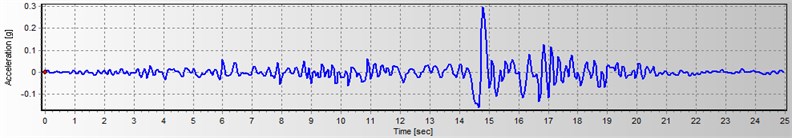
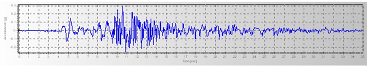
Thus, a wanted some tops can be chosen (The dominant frequencies( for the change of Inverse function Fourier Convert of the acceleration history, as presented in Fig. 1.

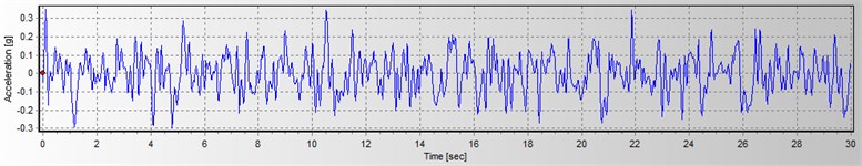
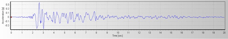
Both the acceleration time history and its FT, as shown in Fig. 1, are associated to one of the registered accelerograms in 1978 in Iran, Tabas, earthquake, that were digitized by a time stage area of 0.01 sec. Following this selection of the required number of peaks meant on the amount of tops closest to the critical original frequencies of the primary method, a characteristic frequency border is examined for the composition of rates around the mountains in the adjusted Inverse function Fourier Convert of the history. Afterward, with taking a larger duration stage such as 0.05 sec, the adjusted Inverse function Fourier Convert of this file is defined, as presented in Fig. 2.

Fig. 1Sample screens show off the PC code for to simplify of digitized accelerograms in that the speedup records in 1978 in Iran, Tabas, earthquake and its FT can be seen in red

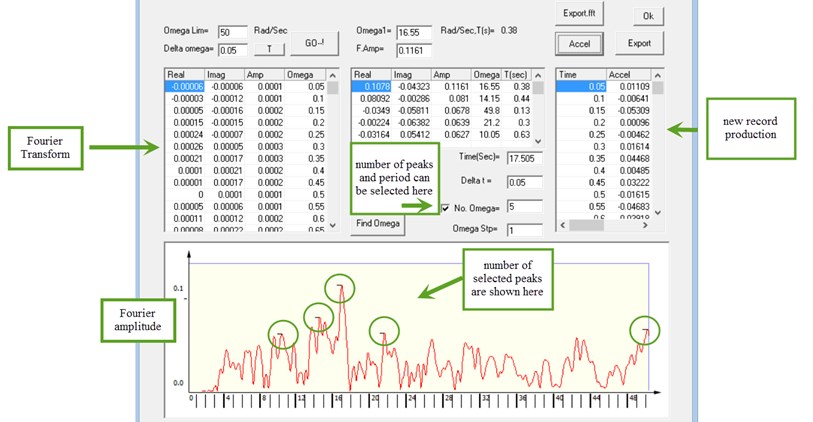
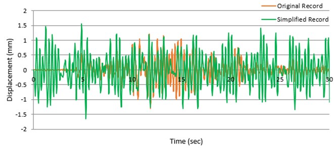
Fig. 2Reduced release of Tabas earthquake by bigger time stages

As observed from a comparison of time histories shown in Figs. 1 and 2, the record reproduced is very different from the primary one. So, get out if this difference has a meaningful effect on the response states, this displacement answer of an SDOF method with a general period of 0.3 sec has been defined by both studies, as presented in Fig. 3.

Fig. 3Answer of model over a time of an SDOF method with average period of 0.3 sec to primary and visible reports in 1978 in Iran, tubas, earthquake

As observed from Fig. 3, these two answers are not in high agreement. As a matter of fact, a contrast to about 25 percent is observed among the two peak answers also the moments of the top answers are not similar.

2.3. Second method for generate acceleration

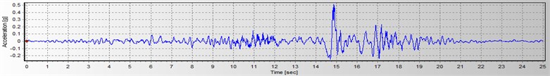
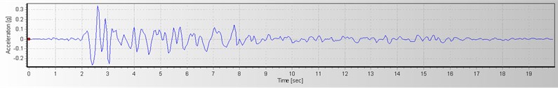
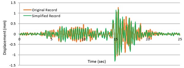
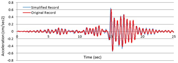
This contrast can be either the result of deletion of some parts of the Fourier Spectrum or selecting a large time step for calculating the Inverse Fourier Transform. To recognize which of these two is the main cause, the full Fourier Spectrum was used (all frequencies) and only a large time step (large distance between $ti$ & $ti+1$) for calculating the Inverse Fourier Transform was applied form equation 7. Fig. 4 shows the results of these computations, applying a duration stage size of 0.05 sec, that is ten times the time stage size of the primary report (0.005 sec) and is linked to one of the accelerograms in 1999, Chi-Chi, Taiwan, earthquake.

Fig. 4a) First a) and b) the visible reports of Chi-Chi, Taiwan, earthquake

a)

b)

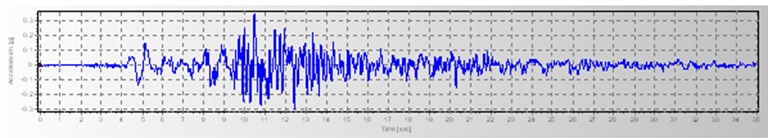
As observed from Fig. 4, nearly similar patterns exist for the two records. However, lower values are observed for the simplified record. This reduction could be due to the use of a larger time step size. Because of these similarities, some simplified records for Tabas and Loma Prieta earthquake records have also been obtained based on the same rule as shown in Figs. 5 and 6.

Fig. 5a) The primary including b) the visible records of Loma Prieta earthquake

a)

b)

2.4. Sample numerical results of linear responses

2.4.1. Build of SDOF structural systems with different time periods

With using a suitable scaling factor, it is reasonable to change the simplified record. The displacement answers of any SDOF methods, with standard intervals of 0.3 to 0.9 sec were limited by both primary and prominent reports of Chi-Chi earthquake to see if the simplified record appears in fair response values.

Fig. 6a) The primary including b) the primary records of Tabas earthquake

a)

b)

2.4.2. Results of structural response

The results of a method with a standard period of 0.3 sec are presented in Fig. 7.

Fig. 7a) Displacement and b) quickening answers of any SDOF method, producing standard time of 0.3 sec determined with primary (presented in red) also visible reports of Chi-Chi, Taiwan, earthquake

a)

b)

Excellent deal exists between the answer values as perceived in Fig. 7. To better observe the amount of differences between the primary and obvious accelerograms, the maximum response rates for this SDOF method with different periods, subjected to the considered earthquake records, both original and simplified, are presented in Table 1.

Table 1 shows that the average amount of differences between peak response values is less than 10 %. As it is unexpectedly observed in Fig. 7, the deal in the state of speedup answers is greater than the event of displacement answers for the SDOF method with an original duration of 0.3 sec. But, it should be chosen out that this is not the case for SDOF methods with other benefits of a standard time.

Table 1Peak response differences between the primary and obvious records of Chi-Chi earthquake

SDOF period (sec)	Time step (sec)	Displacement difference (%)	Acceleration difference (%)
0.3	0.05	10	6
0.5	0.05	6	6
0.7	0.05	9	10
0.9	0.05	12	15
	Average	9.25	9.25

2.4.3. Compare of records spectra

To determine that the agreement is valid in the entire frequency area of the earthquakes, Fourier spectrum, as well as mean speed and false quickening spectra, was compared with both the primary and precise reports. For the accelerogram of the Chi-Chi earthquake and its clear record, examples are shown in Figs. 8 to10 applying a time stage size of 0.05 sec, that is ten times the time stage size of the primary file. Fourier spectrum, as well as low speed and false acceleration spectra, was compared with the initial and precise reports. For the accelerogram of the Taiwan, Chi-Chi, earthquake and its clear report, examples are shown in Figs. 8 to10 applying a time stage size of 0.05 sec, which is ten times the time stage size of the primary file.

Fig. 8Fourier amplitude spectra of the reflected accelerogram of Chi-Chi earthquake measured at both primary and visible records, applying a duration stage size of 0.05 sec (10 periods of the primary file)

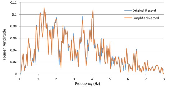
Fig. 9Pseudo velocity spectra of Chi-Chi earthquake measured with both primary and visible reports, utilizing a time stage size of 0.05 sec (10 periods of the primary file)

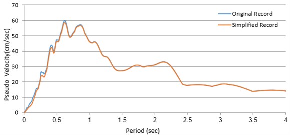
Figs. 8 and 9 show a good match of the Fourier amplitude and pseudo-velocity spectra of the original and the simplified records in the entire frequency range. However, in the pseudo-acceleration spectrum (Figs. 10(a)) a significant difference between the two curves is observed in the low period range. Naturally, using smaller omega intervals (delta omega = 0.01) in the calculation of IFT would lead to a better agreement between the two spectra. (Figs. 10(b)).

Fig. 10Pseudo acceleration spectra of Chi-Chi earthquake measured with both primary and visible reports, utilizing a time stage size of 0.05 sec (10 periods of the primary file)

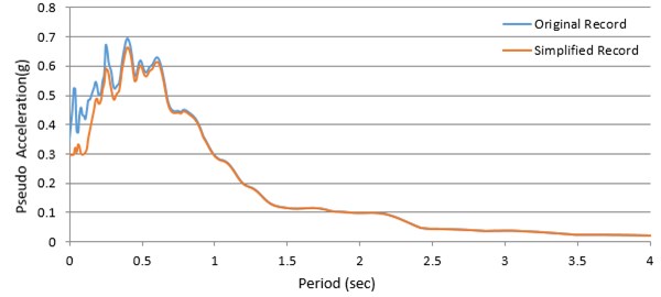
a) Delta omega = 0.05

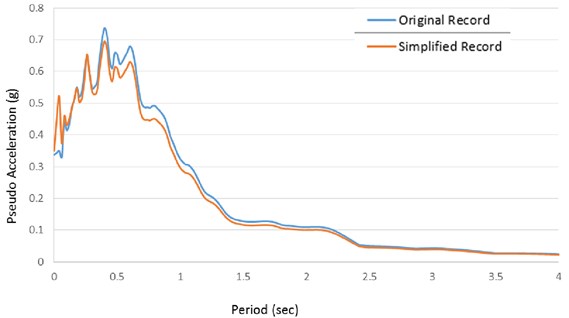
b) Delta omega = 0.01

2.5. Sample numerical results of nonlinear responses

2.5.1. Response of structures

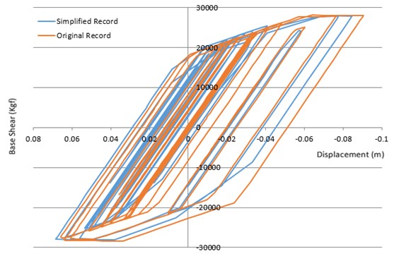
Similar to linear cases, to assess whether the simplified accelerograms result in response values with acceptable precision in nonlinear response analysis. The displacement response and the hysteretic base shear – lateral displacement curves of a set of single degree of freedom (SDOF) systems were determined using both primary and clear records of the selected earthquakes, and the results were compared. Sample results are shown in Figs. 11 to 16.

2.5.2. Result discussion

An excellent agreement between answer charges, obtained by the original and the simplified accelerogram can be observed in Figs. 11 to 16. It can also be found in these figures that the displacement responses obtained by the simplified accelerograms are somewhat higher than those obtained from the original records in cases of all Chi-Chi, Loma Prieta, and Tabas earthquakes. That is also the case for SDOF systems with different amounts of the original period dominated to other earthquakes as well, and this confirms that the intended simplification technique results in conservative responses.

Fig. 11Displacement answer records of the nonlinear SDOF method, having the original period of 0.5 sec, determined by both primary and visible record of Chi-Chi earthquake

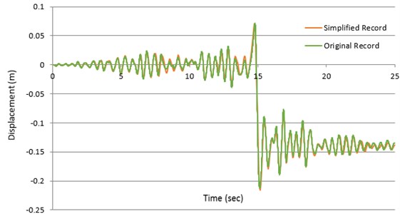
Fig. 12Comparing of hysteretic responses of nonlinear SDOF method, having the original period of 0.5 sec, determined by both primary and visible record of Chi-Chi earthquake

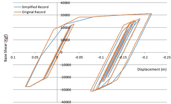
Fig. 13Displacement answer records of the nonlinear SDOF method, having the original period of 0.5 sec, determined by both primary and visible record of Loma Prieta earthquake

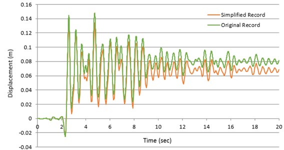
Fig. 14Comparing the hysteretic responses of the nonlinear SDOF method, having the original period of 0.5 sec, determined by both primary and visible record of Loma Prieta earthquake

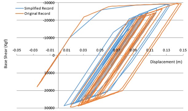
Fig. 15Displacement answer records of the nonlinear SDOF method, having the original period of 0.5 sec, determined by both primary and visible record of Tabas earthquake

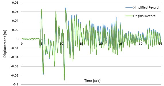
Fig. 16Comparing the hysteretic responses of the nonlinear SDOF method, having the original period of 0.5 sec, determined by both primary and visible record of Tabas earthquake

2.6. Sample numerical results of ida

As the last stage of the study, to ensure the efficiency of the proposed method, the selected original records, and their simplified versions were used in a set of IDA for some SDOF systems. As in the previous sections, there is an excellent agreement in the results of simplified records and original reports as can be observed in Figs. 17 to 19.

Fig. 17IDA curves of nonlinear SDOF method, having the original period of 0.5 sec, determined by both primary and visible record of Chi-Chi earthquake

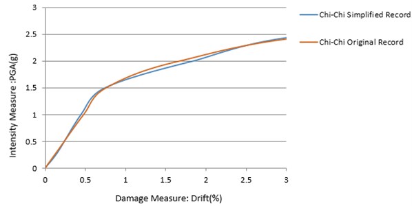
Fig. 18IDA curves of nonlinear SDOF method, having the original period of 0.5 sec, determined by both primary and visible record of Loma Prieta earthquake

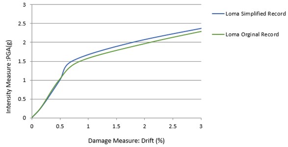
Fig. 19IDA curves of nonlinear SDOF method, having the original period of 0.5 sec, determined by both primary and visible record of Tabas earthquake.

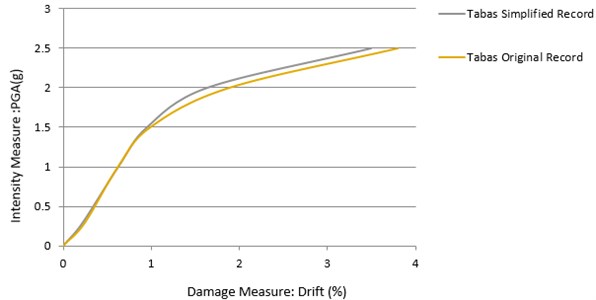
For all these simplified records the time step size is increased to 0.05 sec. For the Chi-Chi and Loma Prieta earthquakes simplified records, this size is tenth times the first time step size, but for the Tabas earthquake, it is as high as five times the original one. Based on Figs. 17 to 19, scaling the records does not have much influence on the results. These results are confirmed results that are discussed in the previous section for hysteretic base shear – lateral displacement curves and movement response histories.

3. Conclusions

As indicated by the numerical results, simplifying the experiences with recording theirs Inverse Fourier Convert applying a time stage extent from five to ten courses that from this primary report leads to just a 5-10 % overestimation of the highest value of displacement and base shear force, related to the natural frequency from that SDOF and the characteristics of the applied records. That is though it reduces the expected response count rate up to 10 times the original amount. Concerning the response spectra, the simplified records result in an absolute decrease of the spectral quickening rates in depressed phase amount. But, in the entire period range, this false speed of the primary and the visible reports are in excellent deal. For IDA, there is also an excellent agreement in the results achieved with simplified and primary records, especially when the simplified documents’ time step size is ten times the original time stage size. By the obtained effects, it can do asserted that the suggested simplification technique is promising for decreasing the calculation costs of nonlinear response of model over time analyses.