Analysis of nonlinear suspension power harvest potential

Zhang, Jin Qiu; Yao, Jun; Zhao, Ming Mei; Li, Xin

doi:10.21595/jve.2017.18329

Journal of Vibroengineering

Browse Journal

Submit article

Published: 31 December 2017

Check for updates

Analysis of nonlinear suspension power harvest potential

Jin Qiu Zhang¹

Jun Yao²

Ming Mei Zhao³

Xin Li⁴

^{1, 2, 3, 4}Academy of Armored Force Engineering Institute, Beijing, China

Corresponding Author:

Jun Yao

Cite the article Download PDF

Downloads 1590

Abstract

Because the power consumption of a controlled suspension is huge, the power harvest potential of a nonlinear controlled suspension is analyzed. Instead of simplifying the suspension to a linear model or adopting some control strategies to solve the problem, this paper investigates the effect of the nonlinear characteristics on the power harvesting potential. A mathematic model is introduced to calculate the nonlinear vibration, and the amount of harvested power was obtained using the multi-scale method. A numerical validation is carried out at the end of this study. The results show that the investigated mechanical parameters affect both the vibration amplitude and the induced current, while the electric parameters only affect the induced current. The power harvesting potential of the nonlinear suspension is generally greater than the linear suspension because the frequency band of the actual pavement also contains bandwidth surrounding the body resonance point. The only exception occurs if the vehicle travels on a road with a particular profile, e.g. a sine curve. To optimize harvested power, it is better to consider the nonlinear characteristics rather than simplifying the suspension to a linear model.

1. Introduction

Power harvesting in nonlinear devices is an important and popular research topic. Nonlinear vibration power harvesting, in particular, has been studied extensively [1-3]. Because the frequency band for which vibration energy can be recycled is wider than for linear vibration, nonlinear vibration devices are widely used to recover vibration energy. A nonlinear device was designed in reference [4] with the axis coil containing a magnetic pole for vibration-energy recovery. An energy recovery device in article [5] contains a mechanical design limit device, which means it is practically a mechanical synchronous switch. Another research group [6] analyzed the effect of external load, external excitation, internal system-parameters, and the equilibrium positions on the dynamic responses of nonlinear tristable energy harvesters. The group found that high-energy interwell oscillations can be achieved in the multi-solution ranges of tristable energy harvesters to improve energy-harvesting from low-level ambient excitations. Several other nonlinear energy-recovery devices have been reported previously [7-9].

Most of these nonlinear vibration-energy recovery devices rely on piezoelectric materials to convert vibration energy into electrical energy. The system parameters in article [10] were optimized globally to maximize the dissipated energy by the nonlinear energy sink and to increase the harvested energy by the piezoelectric element. Article [11] describes nonlinear devices with a spring and beam structure. This structure can increase the deformation of the beam to harvest more power. A linearization method was analyzed in Ref. [12] for nonlinear piezoelectric energy-recovery devices. The numerical simulation shows that this method is effective. Another group [13] studies a random excitation nonlinear vibration-energy harvester potential. Energy recovery of nonlinear vibration with piezoelectric materials were studied in references [14-16]. These studies aim to increase deformation as much as possible, in order to generate more electricity.

Apart from increasing the deformation of piezoelectric materials to obtain more energy, the energy recovery bandwidth can be improved. This includes changing the structure to adjust its resonant frequency [17-20] or employing a structure with two degrees of freedom [21-23]. The nonlinear structure in article [17] was optimized to improve the energy recovery bandwidth. The energy-recovery bandwidth was increased in another study [18] using nonlinear damping. In reference [20], the natural frequency of a nonlinear vibration-energy recovery device can be adjusted, to harvest power near the resonance frequency. Because there are two resonance peaks in a structure with two degrees of freedom, its energy-recovery bandwidth is broader.

However, in certain special circumstances, such as at very high or low frequencies, the energy-recovery efficiency is low. To address this problem, a nonlinear energy-recovery device was designed [24], which is suitable for low frequencies as well as large vibration amplitudes. Some studies [25, 26] focused on nonlinear devices, which are suitable for high-frequency energy-recovery. They attempt to solve energy recovery problems in critical conditions. Other groups investigated 3D printing to manufacture components for nonlinear vibration energy recovery [27], the use of shape memory alloys [28], structures without a spring [29], and other relevant nonlinear vibration-energy recovery related topics [30, 31].

Many nonlinear devices have been very successful, with great applications for low power consumption devices, such as sensors. Studies of large vibration energy harvesting, however, are rare. Vehicle suspension systems are typical nonlinear vibration models with two degrees of freedom. For a controlled suspension system, energy consumption is high, and suspension systems that feature energy recovery are seen as problematic. However, most current research focuses on linearization of the suspension system or the use of different control strategies to facilitate energy recovery. At the same time, this also reduces the bandwidth of energy recovery, which limits further improvement of energy-recovery efficiency. Therefore, in order to make energy recovery more efficient, this work investigates the energy-recovery potential of a suspension system with respect to its nonlinear properties.

2. Governing equations for a nonlinear power-harvesting suspension

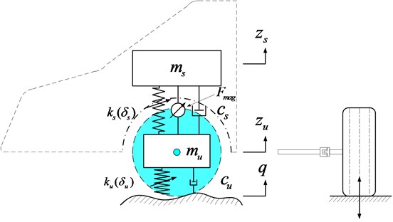
Neglecting complications of a turning vehicle, a suspension model can be described as shown in Fig. 1. The figure includes the sprung mass $m_{s}$ and the unsprung mass $m_{u}$ , which is connected by a nonlinear spring $k_{s} (δ_{s})$ , a shock absorber $c_{s}$ , and an actuator $F_{m a g}$ . The actuator can harvest power when it functions as a generator. Its parameters include magnetic strength $B_{m a g}$ , resistance $R$ , coil length $L_{c o i l}$ , and the coil inductance $L_{i n d}$ . The wheel can be simplified as a nonlinear spring $k_{u} (δ_{u})$ and a damper $c_{u}$ . Excitation from the road is small when a car travels on a freeway, or a construction/military vehicle moves slowly. The unevenness of the ground is considered in the parameter $q$ .

Fig. 1Nonlinear quarter-car model

According to Newton’s second law, the governing equations are:

1a

m_{s} {\ddot{z}}_{s} + f_{c s} ({\dot{z}}_{s} - {\dot{z}}_{s}) + f_{k s} (z_{s} - z_{u}) + f_{m a g} (i) = 0,

1b

m_{u} {\ddot{z}}_{u} - f_{c s} ({\dot{z}}_{s} - {\dot{z}}_{s}) - f_{k s} (z_{s} - z_{u}) - f_{m a g} (i) + f_{c u} ({\dot{z}}_{u} - \dot{q}) + f_{k u} (z_{u} - q) = 0,

1c

L_{i n d} \overset{\cdot}{i} + R i - B_{m a g} L_{c o i l} ({\dot{z}}_{s} - {\dot{z}}_{u}) = 0,

where:

f_{c s} ({\dot{z}}_{s} - {\dot{z}}_{s}) = c_{s} ({\dot{z}}_{s} - {\dot{z}}_{u}), f_{k s} (z_{s} - z_{u}) = k_{s} (z_{s} - z_{u}) + δ_{s} (z_{s} - z_{u})^{3},

f_{m a g} (i) = B_{m a g} L_{c o i l} i, f_{c u} ({\dot{z}}_{u} - \dot{q}) = c_{u} ({\dot{z}}_{u} - \dot{q}),

f_{k u} (z_{u} - q) = k_{u} (z_{u} - q) + δ_{u} (z_{u} - q)^{3} .

Eqs. (1a), (1b), and (1c) can be rewritten as:

2a

\ddot{x} + 2 ς_{x} w_{x} (\dot{x} - \dot{y}) + w_{x}^{2} (x - y) + β_{x} (x - y)^{3} + Γ_{x} i = f c o s (Ω t),

2b

\ddot{y} - 2 ς_{x y} w_{x y} (\dot{x} - \dot{y}) - w_{x y}^{2} x - β_{x y} (x - y)^{3} - Γ_{y} i

+ 2 ς_{y} w_{y} \dot{y} + w_{y}^{2} y + β_{y} y^{3} = f c o s (Ω t),

2c

L_{i n d} \dot{i} + R i - B_{m a g} L_{c o i l} (\dot{x} - \dot{y}) = 0,

where:

z_{s} - q = x, z_{u} - q = y, ς_{x} = \frac{c_{s}}{2 w_{x} m_{s} (τ)}, w_{x}^{2} = \frac{k_{s}}{m_{s} (τ)}, β_{x} = \frac{δ_{s}}{m_{s} (τ)},

ς_{x y} = \frac{c_{s}}{2 w_{x y} m_{u}}, w_{x y}^{2} = \frac{k_{s}}{m_{u}}, β_{x y} = \frac{δ_{s}}{m_{u}}, ς_{y} = \frac{c_{u}}{2 w_{y} m_{u}}, w_{y}^{2} = \frac{k_{s} + k_{u}}{m_{u}}, β_{y} = \frac{δ_{u}}{m_{u}},

Γ_{x} = \frac{B_{m a g} L_{c o i l}}{m_{s}}, Γ_{y} = \frac{B_{m a g} L_{c o i l}}{m_{u}}, - \dot{q} = f c o s (Ω t) .

The sprung mass varies due to load changes. When $m_{s} \approx 9 m_{u} k_{s} / (k_{s} + k_{u})$ , a 3:1 internal resonance occurs.

Because the exact solution for Eq. (2) cannot be found, we use the method of multiple scales to solve the equation. A small perturbation parameter $ε$ is introduced, and a scale transformation is carried out:

3a

ς_{x} \to ε ς_{x}, ς_{x y} \to ε ς_{x y}, β_{x} \to ε β_{x}, β_{x y} \to ε β_{x y}, w_{x y}^{2} x \to ε w_{x y}^{2} x, f \to ε f,

Γ_{x} = ε Γ_{x}, Γ_{y} = ε Γ_{y},

3b

ς_{y} \to ε^{2} ς_{y}, β_{y} \to ε^{2} β_{y} .

Because the stiffness of the tire $k_{u}$ is much bigger, the nonlinearity $δ_{u}$ is much smaller than the spring, the equivalent damping-coefficient $c_{u}$ is much smaller than the damper, and the perturbation parameter is $ε^{2}$ Eq. (3b) after rescaling the stiffness and damping coefficients of the tire in the same equation.

Substituting Eq. (3) into (2) and retaining the $ε^{0}$ and $ε^{1}$ term yields the following equations:

4a

\ddot{x} + 2 ε ς_{x} w_{x} (\dot{x} - \dot{y}) + w_{x}^{2} (x - y) + ε β_{x} (x - y)^{3} + ε Γ_{x} i = ε f c o s (Ω t),

4b

\overset{. .}{y} - 2 ε ς_{x y} w_{x y} (\dot{x} - \dot{y}) - ε w_{x y}^{2} x - ε β_{x y} (x - y)^{3} + w_{y}^{2} y - ε Γ_{y} i = ε f c o s (Ω t),

4c

L_{i n d} \dot{i} + R i - B_{m a g} L_{c o i l} (\dot{x} - \dot{y}) = 0 .

The term $w_{x y}^{2} x$ in Eq. (2b) is much smaller than the term $w_{y}^{2} y$ . Therefore, this term is regarded as a small perturbation term, and it can be rescaled as $ε w_{x y}^{2} x$ in Eq. (4b).

According to the multi scale method, the approximate solution can be expressed as:

5a

x (t, ε) = x_{0} (T_{0}, T_{1}) + ε x_{1} (T_{0}, T_{1}) + O (ε^{2}),

5b

y (t, ε) = y_{0} (T_{0}, T_{1}) + ε y_{1} (T_{0}, T_{1}) + O (ε^{2}), i (t, ε) = i_{0} (T_{0}, T_{1}) + ε i_{1} (T_{0}, T_{1}) + O (ε^{2}),

where $T_{0} = t$ can be seen as faster time scale, and $T_{1} = ε t$ can be seen as slower time scale.

For a 3:1 internal resonance, we can write:

6a

Ω = w_{x} + ε σ,

6b

w_{y} = 3 w_{x} + ε σ_{2},

where $σ$ is a detuning parameter expressing the closeness of $Ω$ to $w_{x}$ , and $σ_{2}$ is a detuning parameter expressing the closeness of $w_{y}$ to $3 w_{x}$ .

We can use the following differential operators:

7a

\frac{d}{d t} (\cdot) = (D_{0} + ε D_{1}) (\cdot), \frac{d^{2}}{d t^{2}} (\cdot) = (D_{0}^{2} + 2 ε D_{0} D_{1}) (\cdot),

7b

D_{0} = \frac{\partial}{\partial T_{0}}, D_{1} = \frac{\partial}{\partial T_{1}} .

Substituting Eqs. (5), (6), and (7) into Eq. (4), and balancing equal powers of $ε$ leads to the following equations:

8a

ε^{0} : D_{0}^{2} x_{0} + w_{x}^{2} x_{0} = w_{y}^{2} y_{0},

8b

D_{0}^{2} y_{0} + w_{y}^{2} y_{0} = 0,

8c

L_{i n d} D_{0} i_{0} + R i_{0} = B_{m a g} L_{c o i l} D_{0} (x_{0} - y_{0}),

9a

ε^{1} : D_{0}^{2} x_{1} + w_{x}^{2} x_{1} = - 2 D_{0} D_{1} x_{0} - 2 ς_{x} w_{x} D_{0} (x_{0} - y_{0})

+ w_{x}^{2} y_{1} - β_{x} (x_{0} - y_{0})^{3} - Γ_{x} i_{0} + f c o s (Ω T_{0}),

9b

\begin{array}{l} D_{0}^{2} y_{1} + w_{y}^{2} y_{1} = - 2 D_{0} D_{1} y_{0} + 2 ς_{x y} w_{x y} D_{0} (x_{0} - y_{0}) + {w_{x y}}^{2} x_{0} + β_{x y} (x_{0} - y_{0})^{3} \\ + Γ_{y} i_{0} + f c o s (Ω T_{0}), \end{array}

9c

L_{i n d} D_{0} i_{1} + R i_{1} = - L_{i n d} D_{1} i_{0} - B_{m a g} L_{c o i l} [D_{1} (x_{0} - y_{0}) + D_{0} (x_{1} - y_{1})] .

The general solution to the Eq. (8) can be expressed as:

10a

x_{0} = G B e^{i w_{y} T_{0}} + G \bar{B} e^{- i w_{y} T_{0}} + A e^{i w_{x} T_{0}} + \bar{A} e^{- i w_{x} T_{0}},

10b

y_{0} = B e^{i w_{y} T_{0}} + \bar{B} e^{- i w_{y} T_{0}},

10c

\begin{array}{l} i_{0} = \frac{B_{m a g} L_{c o i l} (G - 1) i w_{y} B}{R + i w_{y} L_{i n d}} e^{i w_{y} T_{0}} - \frac{B_{m a g} L_{c o i l} (G - 1) i w_{y} \bar{B}}{R - i w_{y} L_{i n d}} e^{- i w_{y} T_{0}} \\ + \frac{B_{m a g} L_{c o i l} i w_{x} A}{R + i w_{x} L_{i n d}} e^{i w_{x} T_{0}} - \frac{B_{m a g} L_{c o i l} i w_{x} \bar{A}}{R - i w_{x} L_{i n d}} e^{- i w_{x} T_{0}} + E (T_{1}) e^{- \frac{R}{L_{i n d}} T_{0}}, \end{array}

where the amplitudes $A$ and $B$ are functions of slower time $T_{1}$ . $\bar{A}$ and $\bar{B}$ are the complex conjugates of $A$ and $B$ , and $G = w_{x}^{2} / (w_{x}^{2} - w_{y}^{2})$ .

Substituting Eq. (10) into (9), and eliminating the secular terms results in the following equations:

11a

\begin{array}{l} - 2 A^{'} i w_{x} - 2 ς_{x} w_{x} A i w_{x} - β_{x} [3 A^{2} \bar{A} + 6 A B \bar{B} (G - 1)^{2} + 3 {\bar{A}}^{2} B (G - 1) e^{i σ_{2} T_{1}}] \\ - Γ_{x} \frac{B_{m a g} L_{c o i l} i w_{x} A}{R + i w_{x} L_{i n d}} + \frac{1}{2} f e^{i σ T_{1}} = 0, \end{array}

11b

\begin{array}{l} - 2 B^{'} i w_{y} - 2 ς_{x y} w_{x y} B i w_{y} + 2 ς_{x y} w_{x y} G B i w_{y} + {w_{x y}}^{2} G B \\ + β_{x y} [6 A \bar{A} B (G - 1) + 3 B^{2} \bar{B} (G - 1)^{3} + A^{3} e^{- i σ_{2} T_{1}}] + Γ_{y} \frac{B_{m a g} L_{c o i l} (G - 1) i w_{y} B}{R + i w_{y} L_{i n d}} = 0, \end{array}

11c

E (T_{1}) = 0 .

Converting $A$ and $B$ into their polar form yields:

12a

A = \frac{1}{2} a e^{i β},

12b

B = \frac{1}{2} b e^{i θ},

where $a$ , $b$ , $β$ and $θ$ are real functions of the slower time $T_{1}$ .

Substituting Eq. (12) into Eq. (11), and separating real and imaginary parts yields the following equations:

13a

a^{'} = - l_{1} a + h_{4} a^{2} b s i n (ϕ - 3 γ) - h_{5} s i n γ,

13b

a γ^{'} = - g_{1} a + h_{6} a^{3} + h_{7} a b^{2} - h_{4} a^{2} b c o s (ϕ - 3 γ) - h_{5} c o s γ,

13c

b^{'} = - l_{2} b + s_{4} a^{3} s i n (ϕ - 3 γ),

13d

b ϕ^{'} = - g_{2} b + s_{5} a^{2} b + s_{6} b^{3} + s_{4} a^{3} c o s (ϕ - 3 γ),

where:

l_{1} = w_{x} ς_{x} + \frac{1}{2} \frac{B_{m a g} L_{c o i l} R}{R^{2} + w_{x}^{2} {L_{i n d}}^{2}} Γ_{x}, h_{4} = - \frac{3}{8} \frac{β_{x}}{w_{x}} (G - 1), h_{5} = \frac{1}{2} \frac{f}{w_{x}},

g_{1} = σ - \frac{1}{2} \frac{B_{m a g} L_{c o i l} w_{x} L_{i n d}}{R^{2} + w_{x}^{2} {L_{i n d}}^{2}} Γ_{x}, h_{6} = \frac{3}{8} \frac{β_{x}}{w_{x}}, h_{7} = \frac{3}{4} \frac{β_{x}}{w_{x}} (G - 1)^{2},

l_{2} = ς_{x y} w_{x y} (1 - G) + \frac{1}{2} \frac{B_{m a g} L_{c o i l} R (G - 1)}{R^{2} + {w_{y}}^{2} {L_{i n d}}^{2}} Γ_{y}, s_{4} = - \frac{1}{8} \frac{β_{x y}}{w_{y}},

g_{2} = 3 σ - σ_{2} + \frac{1}{2} \frac{w_{x y}^{2}}{w_{y}} G - \frac{1}{2} \frac{B_{m a g} L_{c o i l} w_{y} L_{i n d} (G - 1)}{R^{2} + {w_{y}}^{2} {L_{i n d}}^{2}} Γ_{y}, s_{5} = - \frac{3}{4} \frac{β_{x y}}{w_{y}} (G - 1),

s_{6} = - \frac{3 β_{x y}}{8 w_{y}} (G - 1)^{3}, γ = β - σ T_{1}, ϕ = θ + σ_{2} T_{1} - 3 σ T_{1} .

3. Stability analysis of the solutions

The steady-state response of the system can be found by letting $a^{'} = b^{'} =$ 0 and $γ^{'} = ϕ^{'} =$ 0 in Eq. (13):

14a

\begin{array}{l} h_{5}^{2} - l_{1}^{2} a^{2} + \frac{2 l_{2} l_{1} h_{4} b^{2}}{s_{4}} - h_{4}^{2} b^{2} a^{4} - \frac{2 h_{4} (g_{1} - h_{6} a^{2} - h_{7} b^{2}) (g_{2} - s_{5} a^{2} - s_{6} b^{2}) b^{2}}{s_{4}} \\ - (g_{1} - h_{6} a^{2} - h_{7} b^{2})^{2} a^{2} = 0, \end{array}

14b

s_{4}^{2} a^{6} - l_{2}^{2} b^{2} - (g_{2} - s_{5} a^{2} - s_{6} b^{2})^{2} b^{2} = 0 .

There are two kinds of solutions: uncoupled ( $a \neq$ 0 and $b =$ 0), and coupled ( $a \neq$ 0, $b \neq$ 0). In the uncoupled case, Eq. (14) can be simplified as follows:

15

h_{5}^{2} - l_{1}^{2} a^{2} - (g_{1} - h_{6} a^{2})^{2} a^{2} = 0 .

The numbers of solutions for Eq. (15) are 1 or 3. When the intensity of the excitation coming from the road exceeds a certain critical value, there are three solutions. These lead to a saddle node bifurcation and jump in the amplitude/frequency curve. When the excitation intensity is below that critical value, however, only one solution exists. In addition, the critical value can be found when there is only one solution in Eq. (15) for the whole frequency band:

16

h_{5_s t a b l e} = \sqrt{(\frac{8}{3 \sqrt{3}}) (\frac{l_{1}^{3}}{h_{6}})} .

According to Eq. (16), the critical value depends on damping coefficient and nonlinear stiffness of the spring.

Combining Eq (6), (10), and (12) yields:

17a

x = G b c o s (3 Ω t + γ) + a c o s (Ω t + ϕ) + Ο (ε),

17b

y = b c o s (3 Ω t + γ) + Ο (ε),

17c

i = \frac{B_{m a g} L_{c o i l} w_{y}}{\sqrt{R^{2} + {w_{y}}^{2} {L_{i n d}}^{2}}} (G - 1) b c o s (3 Ω t + γ + ϑ_{y})

+ \frac{B_{m a g} L_{c o i l} w_{x}}{\sqrt{R^{2} + {w_{x}}^{2} {L_{i n d}}^{2}}} a c o s (Ω t + ϕ + ϑ_{x}) + Ο (ε),

17d

P = i^{2} R,

where $t a n ϑ_{y} = R / w_{y} L_{i n d}$ , $t a n ϑ_{x} = R / w_{x} L_{i n d}$ .

From Eq. (17) we can see that for the coupled case, two vibration frequencies exist because of internal resonance: a forced vibration frequency ( $Ω$ ) and a free vibration frequency (3 $Ω$ ). The free vibration frequency is exactly three times the forcing frequency. For the uncoupled case, vehicle vibration is mainly reflected by the vibration of sprung mass. Hence, there is only one vibration frequency.

4. Numerical validation

4.1. Frequency response

Let $m_{s} =$ 45 kg, $m_{u} =$ 45 kg, $k_{s} =$ 2000 N/m, $δ_{s} =$ 660 N/m, $k_{u} =$ 16000 N/m. When the damper is inactive, the damping coefficient decreases sharply to $c_{s} =$ 20 Ns/m, then $w_{y} =$ 20 rad/s, $w_{x} =$ 6.6667 rad/s, which leads to $w_{y} \approx 3 w_{x}$ .

According to Eq. (16), the maximum excitation acceleration for which bifurcation does not occur in the steady state is $f_{s t a b l e} = 2 w_{x} h_{5_s t a b l e} =$ 2.05 m/s². When the excitation acceleration increases, the amplitude of the sprung mass vibration will appear as bifurcation caused by the saddle node. In other words, a jump is observed in the amplitude-frequency curve.

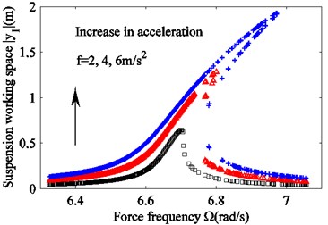
Fig. 2 is obtained from Eq. (15), (17c), (17d) and $b =$ 0. It shows that when the excitation acceleration is below $f_{s t a b l e}$ , the amplitude-frequency curve is single-valued and remains the same for forward and backward frequency sweeping. When the excitation acceleration is much bigger than $f_{s t a b l e}$ , a jump occurs. When the frequency increases, the amplitude is getting higher to reach a maximum before it drops to a much lower level. If the frequency continues to increase, the amplitude decreases. When the frequency decreases, a jump in the opposite direction occurs. In other words, the jump is caused by bifurcation in the amplitude-frequency curve. The curves are different for forward and backward frequency sweeps. With an increase in excitation acceleration, both vibration amplitude of the sprung mass and harvesting power increase for all frequency bands. This is also the case for the unstable frequency band and the band in which energy can be recycled.

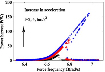
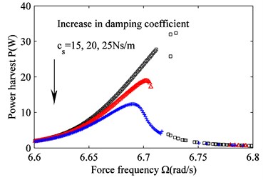
Fig. 3 is obtained from Eq (15), (17c), (17d) and $b =$ 0. It shows the frequency response curve for $f_{s t a b l e} =$ 2.05 m/s². As seen in Fig. 3, when the damping coefficient of the damper exceeds 20 Ns/m, the solution is stable and the steady-state solution of the sprung mass vibration does not bifurcate. On the other hand, bifurcation occurs for the steady-state solution of sprung mass vibration. Furthermore, the smaller the damping coefficient is, the wider the unstable bands become. Unlike the situation shown in Fig. 2, only the amplitude for which the frequency is close to the resonant frequency will become larger when the damping coefficient decreases. Everything else changes little. This indicates that a decreasing nonlinear damping coefficient affects the amplitude for which the frequency is close to the resonant frequency. This increases, both the amplitude and the unstable frequency bands. For the remaining frequency band, the damping coefficient does not affect the amplitude.

Fig. 2The effect of varying acceleration fon the frequency response. a) Suspension working space and b) harvested power. f= 2 m/s2 (black squares), f= 4 m/s2 red triangles), and f= 6 m/s2 (blue crosses)

The effect of varying acceleration fon the frequency response. a) Suspension working space and b) harvested power. f= 2 m/s2 (black squares), f= 4 m/s2 red triangles), and f= 6 m/s2 (blue crosses)

a)

b)

Fig. 3The effect of a varying damping coefficient cs on the frequency response. a) Suspension working space and b) harvested power. cs= 15 Ns/m (black squares), cs= 20 Ns/m (red triangles) and cs= 25 Ns/m (blue crosses)

The effect of a varying damping coefficient cs on the frequency response. a) Suspension working space and b) harvested power. cs= 15 Ns/m (black squares), cs= 20 Ns/m (red triangles) and cs= 25 Ns/m (blue crosses)

a)

b)

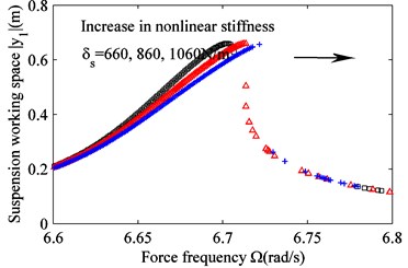
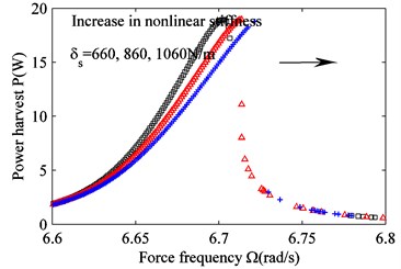
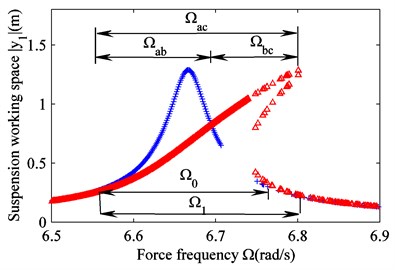
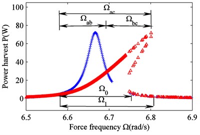
Fig. 4. is obtained from Eqs. (15), (17c), (17d) and $b =$ 0. It shows that the nonlinear stiffness of the spring does not increase the vibration amplitude of the sprung mass; instead, it causes the resonance point to shift to the right and generate unstable bands. The larger the nonlinear stiffness, the wider is the bandwidth for which power is recyclable. In addition, the amount of harvested power increases. Figs. 2, 3, and 4 suggest that both the amplitude of the vibration and the recovered energy depend on the mechanical parameters of the suspension. The increasing acceleration of the excitation, the decreasing nonlinear damping coefficient of the damper, and the increasing nonlinear stiffness of the spring result in increasingly wider and unstable frequency bands. In other words, a larger amount of power can be harvested.

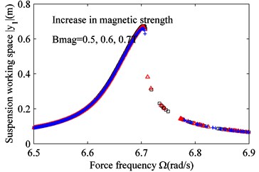
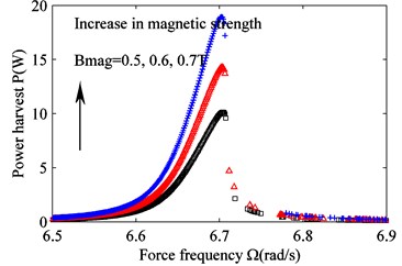
Fig. 5 is obtained from Eqs. (15), (17c), (17d), and $b =$ 0. From Fig. 5 we can see that the effect of magnetic strength on the vehicle vibration amplitude is very small. The vibration curves for different magnetic strengths are very similar for the whole band. The magnetic strength, however, can affect power recovery significantly. The greater the magnetic strength is, the more power the actuator harvests.

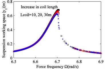
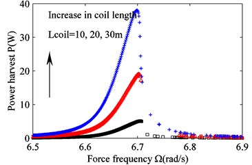
Fig. 6 is obtained from Eqs. (15), (17c), (17d), and $b =$ 0. It shows that the coil length in the actuator affects the vibration amplitude very little. As the coil length increases, the vibration amplitude decreases slightly only near the resonance point. It is essentially the same for the remaining band. The coil length, however, can change the harvested power significantly. The longer the coil length is, the more power the actuator can harvest.

Fig. 4Effect of varying nonlinear stiffness δs on the frequency response. a) Suspension working space and b) harvested power. δs= 660 N/m (black squares), δs= 860 N/m (red triangles) and δs= 1060 N/m (blue crosses)

Effect of varying nonlinear stiffness δs on the frequency response. a) Suspension working space and b) harvested power. δs= 660 N/m (black squares), δs= 860 N/m (red triangles) and δs= 1060 N/m (blue crosses)

a)

b)

Fig. 5The effect of varying magnetic strength Bmag on the frequency response. a) Suspension working space and b) harvested power. Bmag= 0.5 T (black squares), Bmag= 0.6 T (red triangles) and Bmag= 0.7 T (blue crosses)

The effect of varying magnetic strength Bmag on the frequency response. a) Suspension working space and b) harvested power. Bmag= 0.5 T (black squares), Bmag= 0.6 T (red triangles) and Bmag= 0.7 T (blue crosses)

a)

b)

Fig. 6Effect of varying coil length Lcoil on the frequency response. a) Suspension working space and b) harvested power. Lcoil= 10m (black squares), Lcoil= 20 m (red triangles) and Lcoil= 30 m (blue crosses)

Effect of varying coil length Lcoil on the frequency response. a) Suspension working space and b) harvested power. Lcoil= 10m (black squares), Lcoil= 20 m (red triangles) and Lcoil= 30 m (blue crosses)

a)

b)

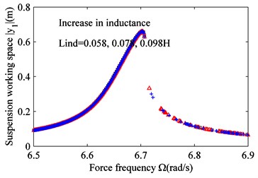
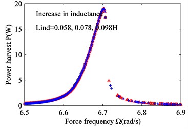
Fig. 7 is obtained from Eqs. (15), (17c), (17d) and $b =$ 0. It indicates that variation of coil inductance has no effect on the vibration amplitude and harvested power.

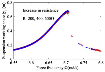
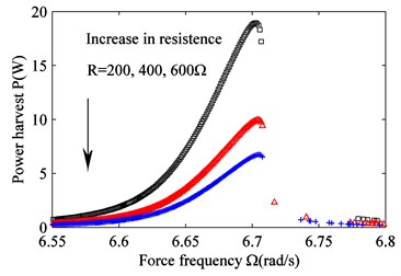
Fig. 8 is obtained from Eqs. (15), (17c), (17d) and $b =$ 0. As seen from Fig. 8, the load resistance affects the vibration amplitude of the vehicle body very little, and the vibration curve for different load resistances is largely the same for the whole frequency band. However, the load resistance can change the harvested power by the actuator. The larger the load resistance, the less power the actuator harvests. According to Figs. 5, 6, 7, and 8, the electrical parameters of the actuator affect the vibration amplitude of the vehicle body hardly. However, they can change the amount of recovered power significantly. If the magnetic strength and the coil length increase, more power can be harvested by the actuator. On the other hand, less power can be harvested when the load resistance increases. The coil inductance, it turns out, affects the power recovery hardly.

Table 1 summarizes how unstable frequency bands, the maximum amplitude of suspension working space, and induced current are affected by the investigated parameters.

Fig. 7Effect of varying coil inductance Lind on frequency response. a) Suspension working space and b) harvested power. Lind= 0.058 H (black squares), Lind= 0.078 H (red triangles), and Lind= 0.098 H (blue crosses)

Effect of varying coil inductance Lind on frequency response. a) Suspension working space and b) harvested power. Lind= 0.058 H (black squares), Lind= 0.078 H (red triangles), and Lind= 0.098 H (blue crosses)

a)

b)

Fig. 8Effect of varying resistance R on the frequency response. a) Suspension working space and b) harvest power. R= 200 Ω (black squares), R= 400 Ω (red triangles) and R= 600 Ω (blue crosses)

Effect of varying resistance R on the frequency response. a) Suspension working space and b) harvest power. R= 200 Ω (black squares), R= 400 Ω (red triangles) and R= 600 Ω (blue crosses)

a)

b)

Table 1Varying trends of result affecting by different parameters

Parameters Results		$f$ (m/s²)	$c_{s}$ (Ns/m)	$δ_{s}$ (N/m)	$B_{m a g}$ (T)	$L_{c o i l}$ (m)	$L_{i n d}$ (H)	$R$ (Ω)
Parameters Results		$↑$	$↑$	$↑$	$↑$	$↑$	$↑$	$↑$
$\|y_{1}\| (m)$	Unstable frequency bands	$↑$	$↓$	$↑$	–	–	–	–
$\|y_{1}\| (m)$	Maximum amplitude	$↑$	$↓$	–	–	–	–	–
$P (w)$	Unstable frequency bands	$↑$	$↓$	$↑$	$↑$	$↑$	–	$↓$
$P (w)$	Maximum amplitude	$↑$	$↓$	–	$↑$	$↑$	–	$↓$
Note: ” $↑$ ” represents an increase; ” $↓$ ” represents a decrease; ”–” represents no change

4.2. Time-domain analysis

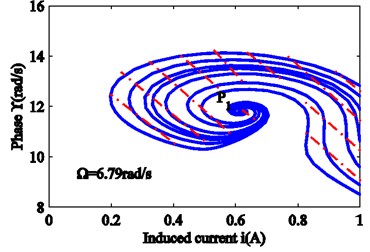
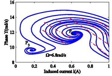
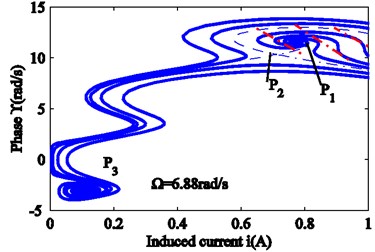
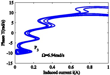
Fig. 9 is obtained from Eqs. (13a), (13b), (17c) and $b =$ 0. The critical lower limit frequency is $w_{d o w n}$ , and the critical upper limit frequency is $w_{u p p e r}$ . When the force frequency $Ω$ approaches $w_{d o w n}$ , all vibrations for the different initial conditions are attracted to the stable focus $P_{1}$ . Once the force frequency $Ω$ satisfies $Ω > w_{d o w n}$ , another stable focus $P_{3}$ generates, which is shown in Figs. 9(a) and 9(b). According to Fig. 9(c), when the force frequency $Ω$ satisfies $w_{d o w n} < Ω < w_{u p p e r}$ , there are two stable focuses $P_{1}$ , $P_{3}$ , and a saddle node $P_{2}$ . Only certain initial values lead to a trajectory that can reach the saddle node $P_{2}$ . For a small disturbance, the system state will move to focus areas $P_{1}$ or $P_{3}$ . The dotted line in Fig. 9(c) is the dividing line between the two regions. The state outside the dotted line moves to the stable focus area $P_{3}$ and the states within the dotted line move to the stable focus area $P_{1}$ . As the force frequency continues to increase, at the time $Ω > w_{u p p e r}$ , the focus area $P_{1}$ disappears, and all states move towards focus area $P_{3}$ . The region covered by the red dashed line changes from large to small, and ultimately disappears. These phenomena indicate that both the upper and the lower two solutions are asymptotically stable in the amplitude frequency curve. The intermediate solution, however, is unstable. Because only asymptotically stable motion can be achieved in the actual physical world, a jump can be seen in the diagram.

Fig. 9Evolution of the phase plane with force frequency: a) 6.79, b) 6.80, c) 6.88, d) 6.94 rad/s

a)

b)

zv

d)

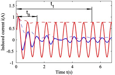
From Eqs. (13a), (13b), and (17c) we can obtain the induced current function $i$ . Since the excitation is described by a sine function, the time domain function $i$ can be written as $i s i n (w_{x} t)$ . As a result, Fig. 10 can be obtained.

Because the steady state of the nonlinear system depends on the initial values, the final stable state with different initial values is different. Because the initial values of the system are not the same, the resulting induced current is different – see Fig. 10. The stable value of the induced current (red curve) is high, and the corresponding stable focus area is $P_{1}$ . Furthermore, the stabilization process requires only a short time $t_{0}$ . The other stable value (blue curve) is small, requiring a longer time $t_{1}$ to become stable. Its corresponding stable focus area is $P_{3}$ . This is consistent with the result shown in Fig. 9, which also confirms that the saddle node $P_{2}$ is impossible to achieve in practice.

Fig. 10Time-domain plot for the induced current

4.3. Comparison with a linear suspension

The difference between the nonlinear system and the linear system is that the bandwidth for which the amplitude exceeds certain critical value is larger for the nonlinear system. Thus, the total amount of recovered energy by nonlinear systems is higher.

Fig. 11Amplitude frequency responses for linear and nonlinear suspensions

a)

b)

Fig. 12Power harvesting potential

a)

b)

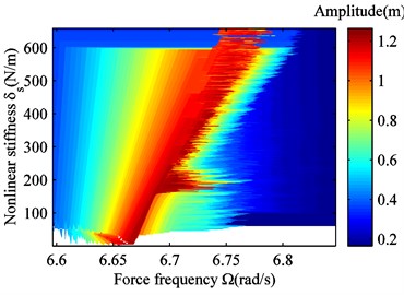
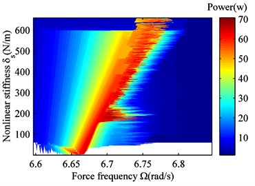
Fig. 11 shows the frequency response curve for linear and nonlinear suspensions with $δ_{s} =$ 660 N/m. When the amplitude exceeds a critical value, the actuator in the suspension can recover energy. Then, the frequency band for the linear suspension (blue curve) is $Ω_{0}$ . The frequency band for the nonlinear suspension is $Ω_{1}$ . It is clear that $Ω_{1} > Ω_{0}$ . Therefore, the energy recovery potential of nonlinear suspensions is greater than that of linear suspensions. The change in the energy-recovery band depends on the nonlinear stiffness. Fig. 12 reflects this change. In Fig. 12, for an increasing nonlinear stiffness, the energy recovery bandwidth increases from 0.21 rad/s ( $δ_{s} =$ 0 N/m) to 0.24 rad/s ( $δ_{s} =$ 660 N/m) for the suspension working space, and 0.18 rad/s ( $δ_{s} =$ 0 N/m) to 0.23 rad/s ( $δ_{s} =$ 660 N/m) for harvested power. However, the change in nonlinear stiffness does not affect the peak value of the vibration amplitude, so the maximum power remains unchanged. However, the peak area moves to the right, and the amount of harvested energy increases.

In addition, from Fig. 11 and Fig. 12 we can see that the energy recovery potential for the nonlinear suspension is greater than for the linear suspension across the whole frequency band $Ω_{a c}$ . For the frequency band $Ω_{a b}$ , the linear suspension energy recovery potential is higher. For the frequency band $Ω_{b c}$ , on the other hand, the nonlinear suspension energy recovery potential is higher. Because the road surface can be considered white noise, the frequency band covers the natural frequency of the vehicle body. This includes $Ω_{a c}$ , and therefore, in reality, the nonlinear suspension energy recovery potential is higher. Further improving the energy recovery potential of nonlinear suspension can increase nonlinear stiffness.

5. Conclusions

For nonlinear suspensions, the damping coefficient of the shock absorber can change the vibration amplitude of the vehicle, and thus affect the magnitude of the induced current. Although nonlinear stiffness does not change the vibration peak, shifting the resonance point to the right changes the bandwidth for the induced current. The electric parameters of the actuator hardly affect the vibration amplitude of the vehicle but they can affect the harvested power significantly. The greater magnetic strength the permanent magnet produces, the longer is the coil and the smaller is the load resistance, and the actuator harvests more power. The inductance of the coil has little effect on the harvested power. Changing these parameters affects the harvested power of the suspension. However, because the nonlinear system is affected by the initial value, the resulting induced current may not be the same-even with the same parameters and different initial conditions. Furthermore, the process to reach the final steady state takes different amounts of time, which also affects the harvested power.

In addition, the power harvest bandwidth for the nonlinear suspension is greater for the whole frequency band. The power harvesting potential of the nonlinear suspension is generally greater because the frequency band of the actual pavement also contains bandwidth surrounding the body resonance point. The only exception occurs if the vehicle travels on a road with a particular profile, e.g. a sine curve.

The harvested power can be increased by increasing the nonlinear stiffness, but this can lead to other problems.

Overall, the energy recovery potential of the nonlinear suspension is greater than that of the linear suspension. To optimize harvested power, it is better to consider the nonlinear characteristics rather than simplifying the suspension to a linear model.

References

Cammarano A., Neild S., Burrow S., Wagg D., Inman D. Optimum resistive loads for vibration-based electromagnetic energy harvesters with a stiffening nonlinearity. Journal of Intelligent Material Systems and Structures, Vol. 25, Issue 14, 2014, p. 1757-1770.

Publisher
Chen L. Q. and Jiang W. A. Internal resonance energy harvesting. Journal of Applied Mechanics, Vol. 82, 2015, p. 1-11.

Publisher
Chen Z. S., Guo B., Xiong Y. P., CHeng C. C., Yang Y. M. Melnikov-method-based broadband mechanism and necessary conditions of nonlinear rotating energy harvesting using piezoelectric beam. Journal of Intelligent Material Systems and Structures, Vol. 27, Issue 18, 2016, p. 2555-2567.

Publisher
Sato T. and Igarashi H. A chaotic vibration energy harvester using magnetic material. Smart Materials and Structures, Vol. 24, 2015, p. 1-8.

Publisher
Wu Y. P., Badel A., Formosa F., Liu W. Q., Agbossou A. Nonlinear vibration energy harvesting device integrating mechanical stoppers used as synchronous mechanical switches. Journal of Intelligent Material Systems and Structures, Vol. 25, Issue 14, 2014, p. 1658-1663.

Publisher
Zhou S. X., Cao J. Y., Inman D. J., Lin J., Li D. Harmonic balance analysis of nonlinear tristable energy harvesters for performance enhancement. Journal of Sound and Vibration, Vol. 373, 2016, p. 223-235.

Publisher
Kremer D., Liu K. A nonlinear energy sink with an energy harvester: transient responses. Journal of Sound and Vibration, Vol. 333, 2014, p. 4859-4880.

Publisher
Ma T., Zhang H. Reaping the potentials of nonlinear energy harvesting with tunable damping and modulation of the forcing functions. Applied Physics Letters, Vol. 104, 2014, p. 1-4.

Publisher
Yildirim T., Ghayesh M. H., Li W. H., Alici G. Design and development of a parametrically excited nonlinear energy harvester. Energy Conversion and Management, Vol. 126, 2016, p. 247-255.

Publisher
Ahmadabadi Z. N., Khadem S. E. Nonlinear vibration control and energy harvesting of a beam using a nonlinear energy sink and a piezoelectric device. Journal of Sound and Vibration, Vol. 333, 2014, p. 4444-4457.

Publisher
Harne R. L., Wang K. W. Axial suspension compliance and compression for enhancing performance of a nonlinear vibration energy harvesting beam system. Journal of Vibration and Acoustics, Vol. 138, 2016, p. 1-10.

Publisher
Jiang W. A., Chen L. Q. An equivalent linearization technique for nonlinear piezoelectric energy harvesters under Gaussian white noise. Communications in Nonlinear Science and Numerical Simulation, Vol. 19, 2014, p. 2897-2904.

Publisher
Paula A. S. D., Inman D. J., Savi M. A. Energy harvesting in a nonlinear piezomagnetoelastic beam subjected to random excitation. Mechanical Systems and Signal Processing, Vol. 54, Issue 55, 2015, p. 405-416.

Publisher
Silva L. L., Savi M. A., Jr P. C. C. M., Netto T. A. On the nonlinear behavior of the piezoelectric coupling on vibration-based energy harvesters. Shock and Vibration, 2015, p. 1-15.

Publisher
Xu J. and Tang J. Multi-directional energy harvesting by piezoelectric cantilever-pendulum with internal resonance. Applied Physics Letters, Vol. 107, 2015, p. 1-5.

Publisher
Zhang Y. S., Zheng R. C., Shimono K., Kaizuka T., Nakano K. Effectiveness testing of a piezoelectric energy harvester for an automobile wheel using stochastic resonance. Sensors, Vol. 16, 2016, p. 1-16.

Publisher
Cammarano A., Neild S. A., Burrow S. G., Inman D. J. The bandwidth of optimized nonlinear vibration-based energy harvesters. Smart Materials and Structures, Vol. 23, 2014, p. 1-9.

Publisher
Tehrani M. C., Elliott S. J. Extending the dynamic range of an energy harvester using nonlinear damping. Journal of Sound and Vibration, Vol. 333, 2014, p. 623-629.

Publisher
Upadrashta D., Yang Y. W. Nonlinear piezomagnetoelastic harvester array for broadband energy harvesting. Journal of Applied Physics, Vol. 120, 2016, p. 1-9.

Publisher
Xie L. H., Du R. X. Frequency tuning of a nonlinear electromagnetic energy harvester. Journal of Vibration and Acoustics, Vol. 136, 2014, p. 1-7.

Publisher
Liu S. G., Cheng Q. J., Zhao D., Feng L. F. Theoretical modeling and analysis of two-degree-of-freedom piezoelectric energy harvester with stopper. Sensors and Actuators A: Physical, Vol. 245, 2016, p. 97-105.

Publisher
Wu H., Tang L. H., Yang Y. W., Soh C. K. Development of a broadband nonlinear two-degree-of-freedom piezoelectric energy harvester. Journal of Intelligent Material Systems and Structures, Vol. 25, Issue 14, 2014, p. 1875-1889.

Publisher
Xiong L. Y., Tang L. H., Mace B. R. Internal resonance with commensurability induced by an auxiliary oscillator for broadband energy harvesting. Applied Physics Letters, Vol. 108, 2016, p. 1-5.

Publisher
Ramezanpour R., Nahvi H., Rad S. Z. A vibration-based energy harvester suitable for low-frequency, high-amplitude environments: Theoretical and experimental investigations. Journal of Intelligent Material Systems and Structures, Vol. 27, Issue 5, 2016, p. 642-665.

Publisher
Remick K., Joo H. K., McFarland D. M., Sapsis T. P., Bergman L., Quinn D. D., Vakakis A. Sustained high-frequency energy harvesting through a strongly nonlinear electromechanical system under single and repeated impulsive excitations. Journal of Sound and Vibration, Vol. 333, 2014, p. 3214-3235.

Publisher
Remick K., Quinn D. D., McFarland D. M., Bergman L., Vakakis A. High-frequency vibration energy harvesting from impulsive excitation utilizing intentional dynamic instability caused by strong nonlinearity. Journal of Sound and Vibration, Vol. 370, 2016, p. 259-279.

Publisher
Bendame M., Rahman E. A., Soliman M. Wideband, low-frequency springless vibration energy harvesters: Part I. Journal of Micromechanics and Microengineering, Vol. 26, 2016, p. 1-12.

Publisher
Constantinou P. and Roy S. A 3D printed electromagnetic nonlinear vibration energy harvester. Smart Materials and Structures, Vol. 25, 2016, p. 1-14.

Publisher
Farsangi M. A. A., Sayyaadi H., Zakerzadeh M. R. A novel inertial energy harvester using magnetic shape memory alloy. Smart Materials and Structures, Vol. 25, 2016, p. 1-9.

Publisher
Joo H. K., Sapsis T. P. Performance measures for single-degree-of-freedom energy harvesters under stochastic excitation. Journal of Sound and Vibration, Vol. 333, 2014, p. 4695-4710.

Publisher
Podder P., Mallick D., Amann A., Roy S. Influence of combined fundamental potentials in a nonlinear vibration energy harvester. Scientific Reports, Vol. 2016, 2016, p. 1-13.

Publisher

About this article

Received

11 March 2017

Accepted

13 June 2017

Published

31 December 2017

SUBJECTS

Vibration generation and control

DOI

https://doi.org/10.21595/jve.2017.18329

Keywords

nonlinear suspension

power harvest

induced current

multi-scale method

stable focus area

Acknowledgements

This research did not receive any specific grant from funding agencies in the public, commercial, or not-for-profit sectors.

This is an open access article distributed under the Creative Commons Attribution License, which permits unrestricted use, distribution, and reproduction in any medium, provided the original work is properly cited.

Previous article in issue Previous Next article in issue Next

Research article

2022 06 30

Nonlinear dynamic analysis of constant-speed and variable-speed of autonomous vehicle passing uneven road

Zhiyong Yang, Long Wang, Fangtao Liu, Zijian Li

Research article

2019 09 30

Optimum suspension design for non-linear half vehicle model using particle swarm optimization (PSO) algorithm

Ahmet Yildiz

Research article

2019 09 30

Collaborative model analysis on ride comfort and handling stability

Yingjie Liu, Dawei Cui

Research article

2019 08 15

Multi-objective optimization of active suspension predictive control based on improved PSO algorithm

Qiang Zhao, Baoquan Zhu

J. Q. Zhang, J. Yao, M. M. Zhao, and X. Li, “Analysis of nonlinear suspension power harvest potential,” Journal of Vibroengineering, Vol. 19, No. 8, pp. 6065–6078, Dec. 2017, https://doi.org/10.21595/jve.2017.18329

Copy Extrica

Copied to clipboard!

TY  - JOUR
DO  - 10.21595/jve.2017.18329
UR  - https://doi.org/10.21595/jve.2017.18329
TI  - Analysis of nonlinear suspension power harvest potential
T2  - Journal of Vibroengineering
AU  - Yao, Jun
AU  - Zhang, Jin Qiu
AU  - Zhao, Ming Mei
AU  - Li, Xin
PY  - 2017
DA  - 2017/12/31
PB  - JVE International Ltd.
SP  - 6065-6078
IS  - 8
VL  - 19
SN  - 1392-8716
ER  - 

Copy Ris

Copied to clipboard!

@article{Yao_2017,
	doi = {10.21595/jve.2017.18329},
	url = {https://doi.org/10.21595/jve.2017.18329},
	year = 2017,
	month = {dec},
	publisher = {{JVE} International Ltd.},
	volume = {19},
	number = {8},
	pages = {6065--6078},
	author = {Jun Yao and Jin Qiu Zhang and Ming Mei Zhao and Xin Li},
	title = {Analysis of nonlinear suspension power harvest potential},
	journal = {Journal of Vibroengineering}
}

Copy Bibtex

Copied to clipboard!

[1]J. Yao, J. Q. Zhang, M. M. Zhao, and X. Li, “Analysis of nonlinear suspension power harvest potential,” Journal of Vibroengineering, vol. 19, no. 8, pp. 6065–6078, Dec. 2017, doi: 10.21595/jve.2017.18329.

Copy IEEE

Copied to clipboard!

Yao, Jun, Jin Qiu Zhang, Ming Mei Zhao, and Xin Li. “Analysis of Nonlinear Suspension Power Harvest Potential.” Journal of Vibroengineering 19, no. 8 (December 31, 2017): 6065–78. https://doi.org/10.21595/jve.2017.18329.

Copy Chicago

Copied to clipboard!

Analysis of nonlinear suspension power harvest potential

Abstract

1. Introduction

2. Governing equations for a nonlinear power-harvesting suspension

3. Stability analysis of the solutions

4. Numerical validation

4.1. Frequency response

4.2. Time-domain analysis

4.3. Comparison with a linear suspension

5. Conclusions

References

About this article

Related Articles