Dynamic analysis and control of strip mill vibration under the coupling effect of roll and rolled piece

Liu, Zhaolun; Jiang, Jiahao; Li, Peng; Pan, Guixiang; Liu, Bin

doi:10.21595/jve.2017.18514

Journal of Vibroengineering

Browse Journal

Submit article

Published: 31 December 2017

Check for updates

Dynamic analysis and control of strip mill vibration under the coupling effect of roll and rolled piece

Zhaolun Liu¹

Jiahao Jiang²

Peng Li³

Guixiang Pan⁴

Bin Liu⁵

^{1, 2, 3}School of Information Science and Engineering, Yanshan University, Qinhuangdao, China

^{4, 5}School of Electrical Engineering, Yanshan University, Qinhuangdao, China

Corresponding Author:

Zhaolun Liu

Cite the article Download PDF

Downloads 1808

WoS Core Citations 5

CrossRef Citations 5

Abstract

According to the “Hill rolling force formula”, taking particular account of the influence from horizontal vibration of rolled piece in roll gap, a dynamic rolling force model is analyzed. Considering the interaction between vibration of strip and roll, the dynamic vibration model of rolling mill is established. On this basis, the time delayed feedback is introduced to control the vibration of the roll system. The amplitude frequency response of the coupled vibration control equation is obtained by using the multiple scales method. Different time delay parameters are selected to test the control effect. Research results show that the unstable vibration of the roll system can be suppressed with appropriate time delay feedback parameters. Because it is simpler and has good control effect in solving nonlinear mechanical vibration, so these results will make a difference for the research of strip mill vibration, and provide theoretical basis for strip steel production.

1. Introduction

Strip steel has been widely used in automobile, aviation, petroleum, chemical industry and so on. It brings great convenience to our life [1]. In fact, the production of strip steel is a very complex process, in which cold rolling is the key step to the quality of strip steel [2]. With the development of society, the surface quality of strip mill has been put forward higher requirements [3]. In cold rolling process, the roll system always happen vibration, so this may leave vibration marks on the surface of strip steel. It will seriously affect the product quality and service life [4, 5].

The research on the vibration of strip rolling mill has lasted for several decades, scholars have done a lot of research from various angles, some of which play a significant role in guiding production. In which, Yun et al. formulated a 2-DOF coupling model by coupling the horizontal vibration and vertical vibration of rolls, then the expression of dynamic component of the rolling force was derived, and they applied it in the mill structure [6, 7]. Noriki et al. investigated the vibration stability of the rolling mill based on a self-excited vibration model; they proposed a high productivity control system aiming at preventing chatter in high speed cold rolling [1, 8]. In Sung’s paper, an adaptive fault compensation control approach was proposed for a class of uncertain nonlinear systems with unknown multiple time-varying delayed nonlinear faults [9, 10]. Zhang et al. researched on the rolling mill vibration caused by flexural-vibration of the strip, and presented an electromechanical coupling vibration model of rolling mill. The unsteady vibration phenomenon has been explained, and importance to the parametric vibration of the rolling mill is attached [11, 12]. Orlowska-Kowalska et al. proposed an adaptive robust control system. The experiment proved that the system had good damping effect and successfully suppressed the torsional vibration of the rolling mill [13]. Fang et al. designed an adaptive synovial variable structure controller to ensure the good stability of the hydraulic servo system, which has a certain inhibitory effect to the vibration of rolling mills [14].

In this paper, considering the effect of horizontal vibration of rolled piece, dynamic vibration model of the roll system is established, and a kind of time delayed feedback is introduced into the vibration system to analyze the roll system. The dynamic characteristics of the roll system are analyzed with different time delay parameters. The simulation results show that the model is effective and feasible. By optimizing the parameters of time delay, the unstable vibration of rolling system can be suppressed.

2. Dynamic formula of rolling force and friction

The rolling force can be calculated by Hill equation as follows [15]:

1

F = B l_{c} Q_{p} K_{T} K,

where:

$B$ – the width of rolled piece;

$l_{c}$ – the contact length between roll and rolled piece in deformation zone, $l_{c} = \sqrt{R Δ h}$ ;

$Q_{p}$ – the influential coefficient in stressed state, $Q_{p} = 1.08 + 1.79 μ ε \sqrt{1 - ε} \sqrt{\frac{R}{H}} - 1.02 ε$ ;

$K_{T}$ – the tension coefficient, $K_{T} = 1 - \frac{0.7 τ_{b} + 0.3 τ_{f}}{K}$ ;

$K$ – the average deformation resistance of materials, $K = 1.15 a_{0} {(\frac{1}{3} ε_{0} + \frac{2}{3} ε_{1})}^{a_{1}}$ ;

$a_{0}$ , $a_{1}$ – the regression coefficient of the model;

$R$ – the work roll radius;

$Δ h$ – reduction quantity of rolled piece, $Δ h = H - h - 2 y$ ;

$H$ – the entrance thickness of rolled piece;

$h$ – the exit thickness of rolled piece;

$y$ – the vibration displacement of rolls;

$ε$ – the reduction rate of rolled piece, $ε = Δ h / H$ ;

$ε_{0}$ – the reduction rate of frame ingress, $ε_{0} = (\bar{H} - H) / \bar{H}$ ;

$ε_{1}$ – the reduction rate of frame egress, $ε_{1} = (\bar{H} - h) / \bar{H}$ ;

$\bar{H}$ – the thickness of pre-rolling rolled piece;

$τ_{f}$ and $τ_{b}$ – the forward and backward tensile stress of rolled piece;

$μ$ is the friction coefficient of roll gap, it may be expressed as follows:

2

μ = \sqrt{\frac{Δ h}{D}} [0.5 + (K_{1} - 0.5) e^{- K_{2} (v_{0} + \dot{x})}],

where, $K_{1}$ and $K_{2}$ are the friction characteristic coefficients; $D$ is the work roll diameter; $v_{0}$ is work roll rotational speed; $\dot{x}$ is the relative vibration speed of rolled piece in roll gap; considering that $K_{2} \cdot \dot{x} ≪ 1$ , so the Roberts equation can be simplified as:

3

μ = μ (0,0) + Δ μ,

where:

\{\begin{array}{l} μ (0,0) = \sqrt{\frac{H - h}{D}} [0.5 + (K_{1} - 0.5) e^{- K_{2} v_{0}}], \\ Δ μ = b_{1} \dot{x} + b_{2} y + b_{3} {\dot{x}}^{2} + b_{4} \dot{x} y + b_{5} y^{2} + b_{6} {\dot{x}}^{3} + b_{7} {\dot{x}}^{2} y + b_{8} \dot{x} y^{2} + b_{9} y^{3}, \end{array}

where:

b_{0} = μ (0,0), b_{1} = \frac{\partial}{\partial \dot{x}} μ (0,0), b_{2} = \frac{\partial}{\partial y} μ (0,0), b_{3} = \frac{1}{2!} \frac{\partial^{2}}{\partial {\dot{x}}^{2}} μ (0,0),

b_{4} = \frac{\partial^{2}}{\partial \dot{x} \partial y} μ (0,0), b_{5} = \frac{1}{2!} \frac{\partial^{2}}{\partial y^{2}} μ (0,0), b_{6} = \frac{1}{3!} \frac{\partial^{3}}{\partial {\dot{x}}^{3}} μ (0,0),

b_{7} = \frac{1}{2} \frac{\partial^{3}}{\partial {\dot{x}}^{2} \partial y} μ (0,0), b_{8} = \frac{1}{2} \frac{\partial^{3}}{\partial y^{2} \partial \dot{x}} μ (0,0), b_{9} = \frac{1}{3!} \frac{\partial^{3}}{\partial y^{3}} μ (0,0) .

When rolling process is stable, $\dot{x} =$ 0, $y =$ 0. Substituting Eq. (2) into Eq. (1), then expanding Eq. (1) at equilibrium point by Taylor equation, the rolling force can be represented as:

4

F = F (0,0) + Δ F,

where:

\{\begin{array}{l} F (0,0) = 1.15 a_{0} B L_{1} L_{2} \sqrt{R H - h}, \\ Δ F = I_{1} \dot{x} + I_{2} y + I_{3} {\dot{x}}^{2} + I_{4} \dot{x} y + I_{5} y^{2} + I_{6} {\dot{x}}^{3} + I_{7} {\dot{x}}^{2} y + I_{8} \dot{x} y^{2} + I_{9} y^{3}, \end{array}

where:

L_{1} = {(\frac{1}{3} ε_{0} + \frac{2}{3} ε_{1})}^{a_{1}} - 0.7 τ_{b} - 0.3 τ_{f},

L_{2} = 1.08 + (1.79 b_{0} e^{- K_{2} v_{0}} \sqrt{h R} - 1.02 H) (\frac{H - h}{H^{2}}), I_{0} = F (0,0), I_{1} = \frac{\partial}{\partial \dot{x}} F (0,0),

I_{2} = \frac{\partial}{\partial y} F (0,0), I_{3} = \frac{1}{2!} \frac{\partial^{2}}{\partial {\dot{x}}^{2}} F (0,0), I_{4} = \frac{\partial^{2}}{\partial \dot{x} \partial y} F (0,0), I_{5} = \frac{1}{2!} \frac{\partial^{2}}{\partial y^{2}} F (0,0),

I_{6} = \frac{1}{3!} \frac{\partial^{3}}{\partial {\dot{x}}^{3}} F (0,0), I_{7} = \frac{1}{2} \frac{\partial^{3}}{\partial {\dot{x}}^{2} \partial y} F (0,0), I_{8} = \frac{1}{2} \frac{\partial^{3}}{\partial y^{2} \partial \dot{x}} F (0,0), I_{9} = \frac{1}{3!} \frac{\partial^{3}}{\partial y^{3}} F (0,0) .

According to the Friction theory, the friction formula can be written as:

5

F_{f} = 2 (μ (0,0) + Δ μ) \times (F (0,0) + Δ F),

where, $μ (0,0)$ and $F (0,0)$ are the steady-state values, $Δ μ$ and $Δ F$ are the dynamic variable quantities; Take the main part of the friction force, Eq. (5) can be written as:

6

Δ F_{f} = 2 μ (0,0) Δ F + 2 Δ μ F (0,0) .

By substituting Eq. (3) and Eq. (4) into Eq. (6), the expression of $Δ F_{f}$ can be obtained:

7

\begin{array}{l} Δ F_{f} = 2 b_{0} [I_{1} \dot{x} + I_{2} y + I_{3} {\dot{x}}^{2} + I_{4} \dot{x} y + I_{5} y^{2} + I_{6} {\dot{x}}^{3} + I_{7} {\dot{x}}^{2} y + I_{8} \dot{x} y^{2} + I_{9} y^{3}] \\ + 2 I_{0} [b_{1} \dot{x} + b_{2} y + b_{3} {\dot{x}}^{2} + b_{4} \dot{x} y + b_{5} y^{2} + b_{6} {\dot{x}}^{3} + b_{7} {\dot{x}}^{2} y + b_{8} \dot{x} y^{2} + b_{9} y^{3}] . \end{array}

3. Coupled vibration control model of strip mill

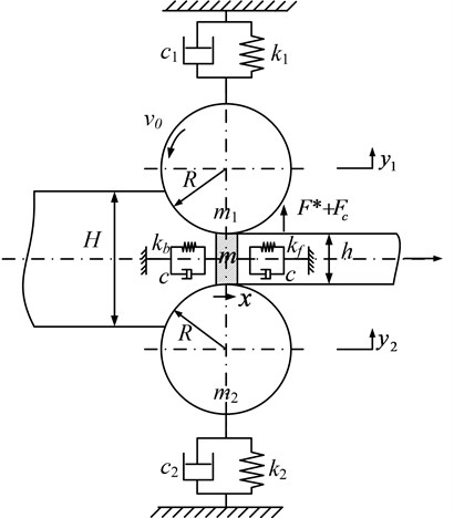
Based on the classic Yun model, considering the influence of the horizontal vibration, the rolling mill coupling vibration model is established as shown in Fig. 1.

In Fig. 1, $m$ is the mass of rolled piece in roll gap, it can be obtained by the equation $m = ρ V$ ; where $ρ$ is the rolled piece density, $V$ is the volume of rolled piece in roll gap, and it may be approximately expressed as:

8

V = \frac{B l_{c} (H + h)}{2} .

The wave force of rolled piece in the forward and backward sliding zones is equivalent to the force function. Its stiffness can be written as:

9

k_{f} = {\frac{τ_{f} S_{f}}{L_{f d}}}_{}, k_{b} = {\frac{τ_{b} S_{b}}{L_{b d}}}_{},

where:

$τ_{f}$ and $τ_{b}$ – forward and backward tension of rolled piece;

$S_{f}$ and $S_{b}$ – forward and backward cross-sectional area of rolled piece;

$L_{f d}$ and $L_{b d}$ – forward and backward deformation length of rolled piece.

$c$ – equivalent damping of the damping effect between the roll and rolled piece;

$m_{1}$ and $m_{2}$ – respectively the equivalent mass of upper and lower rolls;

$k_{1}$ and $k_{2}$ – the equivalent stiffness of upper and lower rolls;

$c_{1}$ and $c_{2}$ – the equivalent dumping of upper and lower rolls;

$y_{1}$ and $y_{2}$ – the vibration displacement of upper and lower rolls;

$F^{*}$ – the external disturbance force of rolls.

Considering the symmetry of mechanical structure and vibration behavior of strip mill, exist $y = (y_{1} + y_{2}) / 2$ , $M = m_{1} = m_{2}$ , $C = c_{1} = c_{2}$ , $K = k_{1} = k_{2}$ .

Based on the generalized dissipation Lagrange principle, the dynamic equilibrium equations along the direction of rolling line and the middle axis are constructed respectively:

10

\{\begin{array}{l} m \ddot{x} + 2 c \dot{x} + (k_{b} + k_{f}) x = 2 b_{0} Δ F + 2 I_{0} Δ μ, \\ M \ddot{y} + C \dot{y} + K y = Δ F + F^{*} + F_{c}, \end{array}

where, $F_{c} = g_{1} y (t - τ_{1}) + g_{2} \dot{y} (t - τ_{2})$ , $F_{c}$ is a function introduced to control unstable vibration of rolling mills because it has good control effect in solving nonlinear mechanical vibration. $g_{1}$ , $g_{2}$ – feedback gain coefficient; $τ_{1}$ , $τ_{2}$ – time delay parameter.

Fig. 1Structure model of strip mill

4. Coupling system solution of strip mill based on time delay feedback

Assuming that the system is subjected to periodic external disturbances, set $F^{*} = F_{0} c o s Ω t$ . By transposition and replacement, Eq. (11) is transformed into a standard form:

11

\{\begin{array}{l} \ddot{x} + ω_{10}^{2} x = ε ({\hat{η}}_{11} Δ F + {\hat{η}}_{12} Δ μ - {\hat{β}}_{1} \dot{x}), \\ \ddot{y} + ω_{20}^{2} y = ε ({\hat{η}}_{21} Δ F + {\hat{η}}_{22} F^{*} - {\hat{β}}_{2} \dot{y} + {\hat{η}}_{23} F_{c}) . \end{array}

In Eq. (11), $ω_{10} = \sqrt{(k_{f} + k_{b}) / m}$ ; ${\hat{η}}_{11} = {\hat{η}}_{12} = 1 / ε m$ ; ${\hat{β}}_{1} = 2 c / ε m$ ; ${\hat{η}}_{21} = {\hat{η}}_{22} = {\hat{η}}_{23} = 1 / ε M$ ; ${\hat{β}}_{2} = C / ε M$ ; $ω_{20} = \sqrt{K / M}$ . $ε$ is a little parameter. For finding a nonlinear approximate solution of Eq. (11), two times scales of $T_{0} = t$ and $T_{1} = ε t$ are selected. By using multiple scales method, set the solution of Eq. (11) as:

12

\{\begin{array}{l} x = x_{0} (T_{0}, T_{1}) + ε x_{1} (T_{0}, T_{1}), \\ y = y_{0} (T_{0}, T_{1}) + ε y_{1} (T_{0}, T_{1}) . \end{array}

Substituting Eq. (12) into Eq. (11) and separating terms of each order of, one has:

13

\{\begin{array}{l} D_{0}^{2} x_{0} + ω_{10}^{2} x_{0} = 0, \\ D_{0}^{2} y_{0} + ω_{20}^{2} y_{0} = 0, \end{array}

14

\{\begin{array}{l} D_{0}^{2} x_{1} + ω_{10}^{2} x_{1} = {\hat{η}}_{11} [\begin{array}{l} I_{1} D_{0} x_{0} + I_{2} y_{0} + I_{3} (D_{0} x_{0})^{2} \\ + I_{4} D_{0} x_{0} y_{0} + I_{5} {y_{0}}^{2} + I_{6} (D_{0} x_{0})^{3} \\ + I_{7} (D_{0} x_{0})^{2} y_{0} + I_{8} D_{0} x_{0} {y_{0}}^{2} + I_{9} {y_{0}}^{3} \end{array}] \\ + {\hat{η}}_{12} [\begin{array}{l} b_{1} D_{0} x_{0} + b_{2} y_{0} + b_{3} (D_{0} x_{0})^{2} \\ + b_{4} D_{0} x_{0} y_{0} + b_{5} {y_{0}}^{2} + b_{6} (D_{0} x_{0})^{3} \\ + b_{7} (D_{0} x_{0})^{2} y_{0} + b_{8} D_{0} x_{0} {y_{0}}^{2} + b_{9} {y_{0}}^{3} \end{array}] - {\hat{β}}_{1} D_{0} x_{0} - 2 D_{0} D_{1} x_{0}, \\ D_{0}^{2} y_{1} + ω_{20}^{2} y_{1} = {\hat{η}}_{21} [\begin{array}{l} I_{1} D_{0} x_{0} + I_{2} y_{0} + I_{3} (D_{0} x_{0})^{2} \\ + I_{4} D_{0} x_{0} y_{0} + I_{5} {y_{0}}^{2} + I_{6} (D_{0} x_{0})^{3} \\ + I_{7} (D_{0} x_{0})^{2} y_{0} + I_{8} D_{0} x_{0} {y_{0}}^{2} + I_{9} {y_{0}}^{3} \end{array}] \\ - {\hat{β}}_{2} D_{0} y_{0} + {\hat{η}}_{22} F_{0} c o s Ω T_{0} - 2 D_{0} D_{1} y_{0} + g_{1} y_{0} (T_{0} - τ_{1}, T_{1} - ε τ_{1}) \\ + g_{2} D_{0} y_{0} (T_{0} - τ_{2}, T_{1} - ε τ_{2}) . \end{array}

The solution of Eq. (13) is setting as:

15

\{\begin{array}{l} x_{0} = A (T_{1}) e^{i ω_{10} T_{0}} + \bar{A} (T_{1}) e^{- i ω_{10} T_{0}}, \\ y_{0} = B (T_{1}) e^{i ω_{20} T_{0}} + \bar{B} (T_{1}) e^{- i ω_{20} T_{0}} . \end{array}

Substituting Eq. (15) into Eq. (14), and system internal resonance is taken into account. By using the small scale detuning parameters, the frequencies are redefined as: $Ω = ω_{20} + ε σ$ ; $ω_{10} = ω_{20} + ε σ_{1}$ . Where, $σ$ and $σ_{1}$ are detuning parameters. To solve Eq. (15), it is convenient to express the solution in polar form:

16

A = \frac{1}{2} a e^{i θ_{1}}, B = \frac{1}{2} b e^{i θ_{2}},

where, $a$ , $b$ , $θ_{1}$ , $θ_{2}$ both are the functions of $T_{1}$ . In order to obtain the solution of equation set, introducing intermediate variables $ϕ,$ $φ;$ define that: $ϕ = θ_{2} - θ_{1} - σ_{1} T_{1};$ $φ = σ T_{1} - θ_{2};$ Substituting $A$ , $B$ , $ϕ$ , $φ$ into Eq. (14), the modulation equations are expressed as:

17

\{\begin{array}{l} D_{0}^{2} x_{1} + ω_{10}^{2} x_{1} = [\begin{array}{l} {\hat{η}}_{11} (I_{1} A i ω_{10} + 3 I_{6} A^{2} \bar{A} i ω_{10}^{3} + 2 I_{8} A B \bar{B} i ω_{10}) \\ + {\hat{η}}_{12} (b_{1} A i ω_{10} + 3 b_{6} A^{2} \bar{A} i ω_{10}^{3} + 2 b_{8} A B \bar{B} i ω_{10}) \\ - {\hat{β}}_{1} A i ω_{10} + 2 D_{1} A i ω_{10} \end{array}] e^{i ω_{10} T_{0}} \\ ∙ [\begin{array}{l} {\hat{η}}_{11} (I_{2} B + 2 I_{7} A \bar{A} B ω_{10}^{2} + 3 I_{9} B^{2} \bar{B}) \\ + {\hat{η}}_{12} (b_{2} B + 2 b_{7} A \bar{A} B ω_{10}^{2} + 3 b_{9} B^{2} \bar{B}) \end{array}] e^{i ω_{20} T_{0}} + \dots + c c, \\ D_{0}^{2} y_{1} + {ω_{20}}^{2} y_{1} = {\hat{η}}_{21} (I_{1} A i ω_{10}^{2} + 3 I_{6} A^{2} \bar{A} i {ω_{10}}^{3} + 2 I_{8} A B \bar{B} i ω_{10}) e^{i ω_{10} T_{0}} \\ ∙ [\begin{array}{l} {\hat{η}}_{21} (I_{2} B + 2 I_{7} A \bar{A} B ω_{10}^{2} + 3 I_{9} B^{2} \bar{B}) \\ - {\hat{β}}_{2} B i ω_{20} - 2 D_{1} B i ω_{20} \end{array}] e^{i ω_{20} T_{0}} + (g_{1} B e^{i ω_{20} τ_{1}} + g_{2} i ω_{20} e^{i ω_{20} τ_{2}}) e^{i ω_{20} T_{0}} \\ + \frac{{\hat{η}}_{22} F_{0}}{2} e^{i Ω T_{0}} + \dots + c c . \end{array}

4.1. System response in the case of primary resonance

In the case of the system main resonance, $ω_{20}$ far away from $ω_{10}$ , $ω_{20}$ infinitely close $Ω$ . Assuming that, $Ω = ω_{20} + ε σ$ , where, $σ$ is the frequency tuning factor. By substituting $Ω$ into Eq. (17) and eliminating the duration of the system, the expression can be obtained

18

\{\begin{array}{l} {\hat{η}}_{11} (I_{1} A i ω_{10} + 3 I_{6} A^{2} \bar{A} i ω_{10}^{3} + 2 I_{8} A B \bar{B} i ω_{10}) \\ + {\hat{η}}_{12} (b_{1} A i ω_{10} + 3 b_{6} A^{2} \bar{A} i ω_{10}^{3} + 2 b_{8} A B \bar{B} i ω_{10}) - {\hat{β}}_{1} A i ω_{10} - 2 D_{1} A i ω_{10} = 0, \\ {\hat{η}}_{21} (I_{2} B + 2 I_{7} A \bar{A} B ω_{10}^{2} + 3 I_{9} B^{2} \bar{B}) - {\hat{β}}_{2} B i ω_{20} - 2 D_{1} B i ω_{20} + g_{1} B e^{i ω_{20} τ_{1}} \\ + g_{2} i ω_{20} e^{i ω_{20} τ_{2}} + \frac{{\hat{η}}_{22} F_{0}}{2} e^{i σ T_{1}} = 0 . \end{array}

In order to solve Eq. (18), the polar coordinates of $A$ , $B$ are introduced:

19

A = \frac{1}{2} a e^{i θ_{1}}, B = \frac{1}{2} b e^{i θ_{2}},

where, $a$ , $b$ , $θ_{1}$ , $θ_{2}$ both are the functions of $T_{1}$ . Introducing intermediate variables $φ$ , set $φ = σ T_{1} - θ_{2}$ . Bring Eq. (19) into Eq. (18), there is:

20

\{\begin{array}{l} {\hat{η}}_{11} (\frac{1}{2} I_{1} a i ω_{10} + \frac{3}{8} I_{6} a^{3} i ω_{10}^{3} + \frac{1}{4} I_{8} a b^{2} i ω_{10}) - \frac{1}{2} {\hat{β}}_{1} a i ω_{10} \\ + {\hat{η}}_{12} (\frac{1}{2} b_{1} a i ω_{10} + \frac{3}{8} b_{6} a^{3} i ω_{10}^{3} + \frac{1}{4} b_{8} a b^{2} i ω_{10}) - \dot{a} i ω_{10} + {\dot{θ}}_{1} a ω_{10} = 0, \\ {\hat{η}}_{21} (\frac{1}{2} I_{2} b + \frac{1}{4} I_{7} a^{2} b {ω_{10}}^{2} + \frac{3}{8} I_{9} b^{3}) - \frac{1}{2} {\hat{β}}_{2} b i ω_{20} - \dot{b} i ω_{20} + {\dot{θ}}_{2} b ω_{20} \\ + \frac{1}{2} g_{1} b e^{i ω_{20} τ_{1}} + \frac{1}{2} g_{2} b i ω_{20} e^{i ω_{20} τ_{2}} + \frac{{\hat{η}}_{22} F_{0}}{2} e^{i φ} = 0 . \end{array}

The Eq. (20) are expanded into the real and imaginary parts, and then the parameters at the two ends of the equation are equal:

21

\{\begin{array}{l} \dot{a} = {\hat{η}}_{11} (\frac{1}{2} I_{1} a + \frac{3}{8} I_{6} a^{3} ω_{10}^{2} + \frac{1}{4} I_{8} a b^{2}) - \frac{1}{2} {\hat{β}}_{1} a \\ + {\hat{η}}_{12} (\frac{1}{2} b_{1} a + \frac{3}{8} b_{6} a^{3} ω_{10}^{2} + \frac{1}{4} b_{8} a b^{2}), \\ {\dot{θ}}_{1} a = 0, \\ {\dot{θ}}_{2} b = - \frac{{\hat{η}}_{21}}{ω_{20}} (\frac{1}{2} I_{2} b + \frac{1}{4} I_{7} a^{2} b ω_{10}^{2} + \frac{3}{8} I_{9} b^{3}) \\ + \frac{1}{2 ω_{20}} g_{1} b c o s ω_{20} τ_{1} + \frac{1}{2} g_{2} b s i n ω_{20} τ_{2} - \frac{{\hat{η}}_{22} F_{0}}{2 ω_{20}} c o s φ, \\ \dot{b} = - \frac{1}{2} {\hat{β}}_{2} b + \frac{1}{2 ω_{20}} g_{1} b s i n ω_{20} τ_{1} + \frac{1}{2} g_{2} b c o s ω_{20} τ_{2} + \frac{{\hat{η}}_{22} F_{0}}{2 ω_{20}} s i n φ . \end{array}

When the rolling system is stable, $\dot{a} = \dot{b} =$ 0; ${\dot{θ}}_{1} = {\dot{θ}}_{2} =$ 0. The main resonance amplitude frequency equation of the system is obtained after the elimination of $φ$ :

22

\begin{array}{l} {[\frac{2 {\hat{η}}_{21}}{ω_{20}} ζ + \frac{1}{ω_{20}} g_{1} b c o s ω_{20} τ_{1} + g_{2} b s i n ω_{20} τ_{2}]}^{2} \\ + {({\hat{β}}_{2} b + \frac{1}{ω_{20}} g_{1} b s i n ω_{20} τ_{1} + g_{2} b c o s ω_{20} τ_{2})}^{2} = {(\frac{{\hat{η}}_{22} F_{0}}{ω_{20}})}^{2}, \end{array}

where:

ζ = \frac{1}{2} I_{2} b + \frac{1}{4} I_{7} a^{2} b ω_{10}^{2} + \frac{3}{8} I_{9} b^{3}, a^{2} = \frac{{\hat{η}}_{11} (4 I_{1} + 2 I_{8} b^{2}) - 4 {\hat{β}}_{1} + {\hat{η}}_{12} (4 b_{1} + 2 b_{8} b^{2})}{3 {ω_{10}}^{2} (I_{6} {\hat{η}}_{11} + b_{6} {\hat{η}}_{12})} .

4.2. System response in the case of Internal resonance

Considering the case of the system internal resonance, set, $Ω = ω {}_{20} + ε σ;$ $ω_{10} = ω_{20} + ε σ_{1}$ . $σ$ and $σ_{1}$ are the frequency tuning factor. In order to avoid the term in the equation, it must meet:

23

\{\begin{array}{l} {\hat{η}}_{11} (\begin{matrix} I_{1} A i ω_{10} + I_{2} B e^{- i σ_{1} T_{1}} + 3 I_{6} A^{2} \bar{A} i ω_{10}^{3} \\ + 2 I_{7} A \bar{A} B ω_{10}^{2} e^{- i σ_{1} T_{1}} + 2 I_{8} A B \bar{B} i ω_{10} + 3 I_{9} B^{2} \bar{B} e^{- i σ_{1} T_{1}} \end{matrix}) \\ + {\hat{η}}_{12} (\begin{matrix} b_{1} A i ω_{10} + b_{2} B e^{- i σ_{1} T_{1}} + 3 b_{6} A^{2} \bar{A} i {ω_{10}}^{3} \\ + 2 b_{7} A \bar{A} B ω_{10}^{2} e^{- i σ_{1} T_{1}} + 2 b_{8} A B \bar{B} i ω_{10} + 3 b_{9} B^{2} \bar{B} e^{- i σ_{1} T_{1}} \end{matrix}) \\ \begin{array}{l}  \end{array} - {\hat{β}}_{1} A i ω_{10} - 2 D_{1} A i ω_{10} = 0, \\ {\hat{η}}_{21} (\begin{matrix} I_{1} A i ω_{10} e^{i σ_{1} T_{1}} + I_{2} B + 3 I_{6} A^{2} \bar{A} i ω_{10}^{3} e^{i σ_{1} T_{1}} \\ + 2 I_{7} A \bar{A} B ω_{10}^{2} + 2 I_{8} A B \bar{B} i ω_{10} e^{i σ_{1} T_{1}} + 3 I_{9} B^{2} \bar{B} \end{matrix}) \\ \begin{array}{l}  \end{array} - \hat{β} {}_{2} B i ω_{20} + \frac{{\hat{η}}_{22} F_{0}}{2} e^{i σ_{1} T_{1}} - 2 D_{1} B i ω_{20} + g_{1} B e^{- i ω_{20} τ_{1}} + g_{2} B i ω_{20} e^{- i ω_{20} τ_{2}} = 0 . \end{array}

The Eq. (23) are expanded into the real and imaginary parts, and then the parameters at the two ends of the equation are equal:

24

\{\begin{array}{l} \dot{a} = \frac{{\hat{η}}_{11}}{ω_{10}} ψ + \frac{{\hat{η}}_{12}}{2} E - \frac{1}{2} {\hat{β}}_{1} a + [\frac{{\hat{η}}_{11}}{ω_{10}} ζ + \frac{{\hat{η}}_{12}}{ω_{10}} F] s i n φ, \\ a (\dot{φ} + \dot{ϕ}) = [\frac{{\hat{η}}_{11}}{ω_{10}} ζ + \frac{{\hat{η}}_{12}}{ω_{10}} F] c o s φ + a (σ - σ_{1}), \\ \dot{b} = \frac{{\hat{η}}_{21}}{ω_{20}} ψ c o s φ - \frac{1}{2} \hat{β} {}_{2} b + \frac{1}{2 ω_{20}} g_{2} b c o s ω_{20} τ_{2} - \frac{1}{2} g_{1} b s i n ω_{20} τ_{2} + \frac{{\hat{η}}_{22} F_{0}}{2 ω_{20}} s i n ϕ, \\ b \dot{ϕ} = \frac{{\hat{η}}_{21}}{ω_{20}} (ψ s i n φ + ζ) + \frac{{\hat{η}}_{22} F_{0}}{2 ω_{20}} c o s ϕ + \frac{1}{2} g_{1} b c o s ω_{20} τ_{2} - \frac{1}{2 ω_{20}} g_{2} b s i n ω_{20} τ_{2} + b σ, \\ \begin{array}{l}  \end{array} \end{array}

where:

E = b_{1} a + \frac{3}{4} b_{6} a^{3} ω_{10}^{2} + \frac{1}{2} b_{8} a b^{2} F = \frac{1}{2} b_{2} b + \frac{1}{4} b_{7} a^{2} b ω_{10}^{2} + \frac{3}{8} b_{9} b^{3},

ψ = \frac{1}{2} I_{1} a ω_{10} + \frac{3}{8} I_{6} a^{3} ω_{10}^{3} + \frac{1}{4} I_{8} a b^{2} ω_{10} ζ = \frac{1}{2} I_{2} b + \frac{1}{4} I_{7} a^{2} b ω_{10}^{2} + \frac{3}{8} I_{9} b^{3} .

When the rolling system is stable, there is, $\dot{a} = \dot{b} =$ 0; ${\dot{θ}}_{1} = {\dot{θ}}_{2} =$ 0; The main resonance amplitude frequency equation of the system is obtained after the elimination of $φ$ and $φ$ :

25

{[\frac{{\hat{η}}_{11}}{ω_{10}} ψ + \frac{{\hat{η}}_{12} E}{2} - \frac{{\hat{β}}_{1} a}{2}]}^{2} + {[a (σ - σ_{1})]}^{2} = {[\frac{{\hat{η}}_{11} ζ + {\hat{η}}_{12} F}{ω_{10}}]}^{2},

26

\begin{array}{l} {[\frac{2 {\hat{η}}_{21}}{ω_{20}} (ψ s i n φ + ζ) + 2 b σ + \frac{g_{1} b}{ω_{20}} c o s ω_{20} τ_{2} - g_{2} b s i n ω_{20} τ_{2}]}^{2} \\ + {[\frac{2 {\hat{η}}_{21}}{ω_{20}} ψ c o s φ + g_{2} b c o s ω_{20} τ_{2} - \frac{g_{1} b}{ω_{20}} s i n ω_{20} τ_{2} - {\hat{β}}_{2} b]}^{2} = {(\frac{{\hat{η}}_{22} F_{0}}{ω_{20}})}^{2}, \end{array}

where:

c o s φ = \frac{- a ω_{10} (σ - σ_{1})}{{\hat{η}}_{11} ζ + {\hat{η}}_{12} F}, s i n φ = - \frac{2 {\hat{η}}_{11} ψ + {\hat{η}}_{12} ω_{10} E - ω_{10} {\hat{β}}_{1} a}{2 {\hat{η}}_{11} ζ + 2 {\hat{η}}_{12} F} .

5. Characteristic analysis and control of strip mill

Selecting the actual parameters of 1780 mm rolling mill of Chengde Iron and Steel Co., Ltd as an example. The characteristic of coupling vibration model is numerically analyzed. The corresponding system parameters in the model are shown in Table 1.

5.1. Vibration time domain control of rolling mill system

The vibration of the rolling mill system is very likely to occur high frequency self-excited vibration because of its sudden and divergent characteristics. If the vibration divergence behavior of the mill the roll system is controlled, the limit cycle amplitude of the mill the roll system converges to a small range, which enhances the stability of the system to a certain extent. Based on this, the control effect of the stability of the limit cycle amplitude of the roller system vibration is tested.

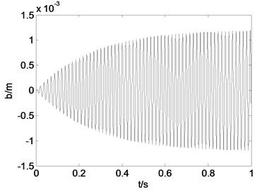
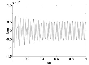
Fig. 2 shows the time history curve and phase diagram of noncontrolled system.

Fig. 3 shows the time history curve and phase diagram when $g_{1} =$ 10000, $g_{2} =$ 50, $τ_{1} =$ 0.75 $T$ , $τ_{2} =$ 0.

Table 1Parameters of rolling mill system

Parameters	Values
Mass of up rolls ( $M$ )	1.44×10⁵ kg
Stiffness of up rolls ( $K$ )	2.08×10⁶ N/m
Damping of up rolls ( $C$ )	1.04×10⁶ N·s/m
Mass of rolled piece ( $m$ )	0.6318 kg
Forward stiffness of rolled piece ( $k_{f}$ )	7.58×10⁷ N/m
Backward stiffness of rolled piece ( $k_{b}$ )	1.10×10⁸ N/m
Damping of rolled piece ( $c$ )	5.20×10³ N·s/m
Width of rolled piece ( $B$ )	1.5 m
Amplitude of external excitation ( $F_{0}$ )	0.5 MN
Thickness of pre-rolling rolled piece ( $\bar{H}$ )	0.0145 m
Entrance thickness of rolled piece ( $H$ )	0.0141 m
Exit thickness of rolled piece ( $h$ )	0.0082 m
Rotational speed of work roll ( $v_{0}$ )	2.5 m/s
Roll diameter ( $D$ )	0.84 m
Density of rolled piece ( $ρ$ )	7.8×10³ kg·m^-3
Forward tension of rolled piece ( $τ_{f}$ )	3.8 MPa
Backward tension of rolled piece ( $τ_{b}$ )	5.5 MPa

Fig. 2Time history curve and phase diagram of noncontrolled system

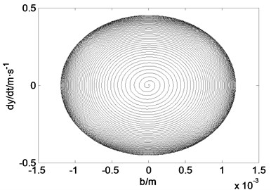
a) Time history curve

b) Phase diagram

Fig. 3Time history curve and phase diagram when g1= 10000, g2= 50, τ1= 0.75T, τ2= 0

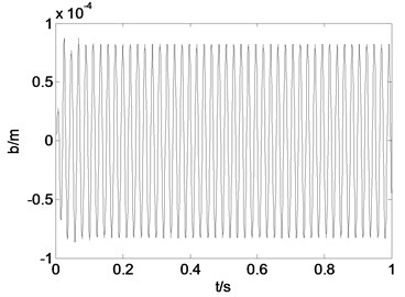
a) Time history curve

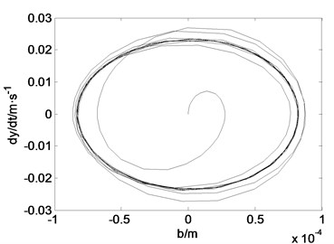
b) Phase diagram

Fig. 4 shows the time history curve and phase diagram when $g_{1} =$ 15000, $g_{2} =$ 50, $τ_{1} =$ 0, $τ_{2} =$ 0.75 $T$ . It can be seen from the comparison of the simulation results that the vibration amplitude of the system without the feedback function increases slowly at the moment of oscillation and finally reaches a stable oscillation, and the amplitude and the convergence of the system introduced the delayed feedback control function can be improved by adjusting the gain coefficient and the time delay. In the case of $g_{1} =$ 10000, $g_{2} =$ 50, $τ_{1} =$ 0.75 $T$ , $τ_{2} =$ 0, the vibration amplitude of the roll system of the rolling mill is similar to that of the constant amplitude oscillation, and the vibration amplitude of the system is reduced and the amplitude of the limit cycle is stable. In the case of $g_{1} =$ 15000, $g_{2} =$ 50, $τ_{1} =$ 0, $τ_{2} =$ 0.75 $T$ , the vibration amplitude of the roll system of the rolling mill is convergent and the amplitude of the limit cycle is stable, and the vibration amplitude of the roller system is further reduced.

Fig. 4Time history curve and phase diagram when g1= 15000, g2= 50, τ1= 0, τ2= 0.75T

a) Time history curve

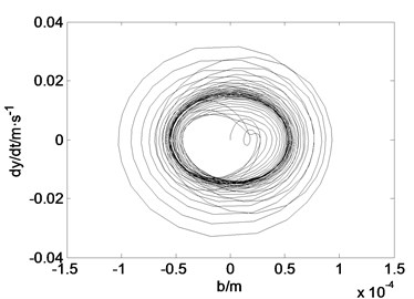
b) Phase diagram

5.2. Vibration amplitude frequency control of rolling mill system

In the amplitude frequency curve, if the amplitude frequency curve jumps, the amplitude of the system will be switched back and forth at the same frequency, which is not conducive to the stable operation of the system. In order to avoid the jumping phenomenon of the amplitude frequency curve of the mill the roll system, the velocity feedback gain coefficient and the time delay parameters are adjusted to eliminate the vibration of the roller system.

Fig. 5Amplitude frequency curve with g1

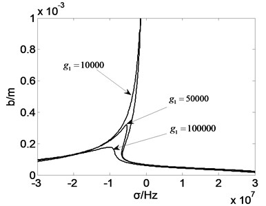
Fig. 6Amplitude frequency curve with g2

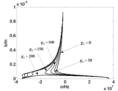
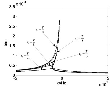
It can be seen from the simulation results that with the change of the feedback parameters, the jump phenomenon of the roller vibration amplitude will be changed to some extent. Fig. 5 shows that with increasing of the displacement feedback gain coefficient $g_{1}$ , the amplitude of vibration of rolls along the ridge and valley line decreases, when the value of $g_{1}$ orders of magnitude greater than 105, rolling mill vibration amplitude jump phenomenon disappeared. Fig. 6 shows that when the value of $g_{2}$ is 200, the phenomenon of “jump” disappears. However, when the $g_{2}$ value is between 0-200, the vibration amplitude decreases. The frequency range of the jumping phenomenon in the roll system of rolling mill increases, and the stability of the system is weakened. Fig. 7 shows that the changes of the parameters $τ_{1}$ delay will not only change the rolling mill vibration amplitude, the frequency interval will influence the natural frequency of vibration of rolling mill rolls and jump phenomenon. Fig. 8 shows that compared to the effect of $τ_{1}$ , the change of $τ_{2}$ did not change the natural frequency of vibration mill. With $τ_{2}$ changes, rolling mill vibration amplitude along the ridge and valley line becomes larger or reduced, when $τ_{2} =$ 0.5 $T$ , the system jump phenomenon disappeared, rolling system restore stability. The parameters in $F c$ work together when one parameter changes, the other three parameters are fixed value but not zero. Any other one parameter is zero, it will affect the overall control effect of the system.

Fig. 7Amplitude frequency curve with τ1

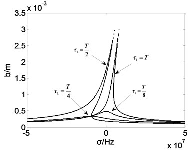
Fig. 8Amplitude frequency curve with τ2

5.3. Bifurcation stability control of main resonance of rolling mill the roll system

Elimination of Eq. (22) in the $a$ , get:

27

c_{1} b^{6} + c_{2} b^{4} + c_{3} b^{2} + c_{4} = 0,

where:

c_{1} = {[\frac{{\hat{η}}_{21}}{ω_{20}} (\frac{{\hat{η}}_{11} I_{7} I_{8} + 2 {\hat{η}}_{12} I_{7} b_{8}}{12 (I_{6} {\hat{η}}_{11} + b_{6} {\hat{η}}_{12})} + \frac{3}{8} I_{9})]}^{2}, c_{4} = - {(\frac{{\hat{η}}_{22} F_{0}}{2 ω_{20}})}^{2},

c_{2} = \frac{{\hat{η}}_{21}^{2}}{{ω_{20}}^{2}} (\frac{{\hat{η}}_{11} I_{7} I_{8} + 2 {\hat{η}}_{12} I_{7} b_{8}}{12 (I_{6} {\hat{η}}_{11} + b_{6} {\hat{η}}_{12})} + \frac{3}{8} I_{9}) \times (\begin{array}{l} I_{2} b + \frac{2 {\hat{η}}_{11} I_{7} I_{1} - 2 {\hat{β}}_{1} I_{7} + 2 {\hat{η}}_{12} b_{1} I_{7}}{3 (I_{6} {\hat{η}}_{11} + b_{6} {\hat{η}}_{12})} \\ + \frac{1}{2 ω_{20}} g_{1} c o s ω_{20} τ_{1} + \frac{1}{2} g_{2} s i n ω_{20} τ_{2} \end{array}),

c_{3} = {[\frac{{\hat{η}}_{21}}{ω_{20}} (\frac{1}{2} I_{2} b + \frac{4 {\hat{η}}_{11} I_{7} I_{1} - 4 {\hat{β}}_{1} I_{7} + 4 {\hat{η}}_{12} b_{1} I_{7}}{12 (I_{6} {\hat{η}}_{11} + b_{6} {\hat{η}}_{12})})]}^{2} + {(\frac{1}{2} {\hat{β}}_{2} b + \frac{1}{2 ω_{20}} g_{1} s i n ω_{20} τ_{1} + \frac{1}{2} g_{2} c o s ω_{20} τ_{2})}^{2} .

Divide both ends of the type (27) at the same time by $c_{1}$ , the standard form is:

28

z^{6} + α z^{4} + β z^{2} + μ = 0,

where:

α = \frac{c_{2}}{c_{1}}, β = \frac{c_{3}}{c_{1}}, μ = \frac{c_{4}}{c_{1}} .

According to the Singularity theory, Eq. (28) is the universal unfolding of the paradigm $g (z, μ) = z^{6} + μ =$ 0, the transfer of the system is Bifurcation set: $B_{0} = B_{1} = Φ$ ;

Lag point set: $H_{0} = \{β = 0\}$ ; $H_{1} = \{α^{2} - 3 β = 0; α \leq 0\}$ ;

Double limit point set: $D = \{α^{2} - 4 β = 0; α \leq 0\}$ ;

Transition set of the system is: $\sum = B_{0} \cup B_{1} \cup H_{0} \cup H_{1} \cup D$ .

The transition set of the system is calculated by MATLAB, and the region of the transfer set is shown in Fig. 9. It can be seen from the Fig. 9 that the 3 boundary of the transfer set divides the system into two real parameter regions. Selecting a representative point in the 3 borderline and 3 sub regions, the corresponding bifurcation topology of the system is analyzed, as shown in Fig. 10.

Fig. 9Transition sets of the system parameters

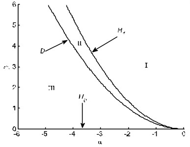
Fig. 10Bifurcation diagram of the system

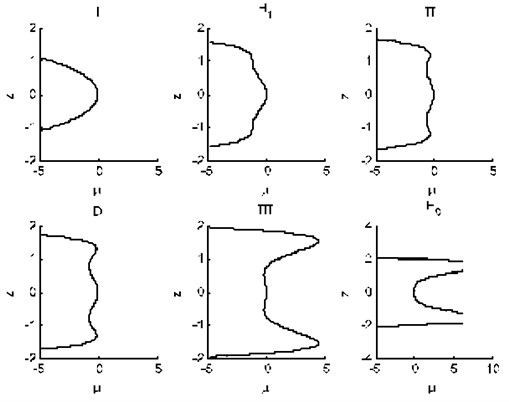
It can be seen from the Fig. 9 and Fig. 10 that the topological diagram of the system bifurcation presents the stable state of the unique solution when the combination of the opening and closing parameters is in the region $Ι$ . When the combination of the opening and closing parameters of the system passes through the critical state of the $H_{1}$ , the vibration amplitude of the roller system become unstable; When the bifurcation parameter is near the zero value, the amplitude of the roll system of the rolling mill jumps several times. After the opening and closing parameters enter the parameter III region through the critical state of the bipolar line point set $D$ , the bifurcation parameter interval of the vibration amplitude of the roller system is gradually expanded. At the same time, the vibration amplitude of the mill the roll system in response to the parameter is in the positive range of bifurcation parameter. In this region, the rolling mill vibration system becomes more sensitive to the change of the opening parameters.

The transition set and bifurcation topology of the system without control are also shown in Fig. 9 and Fig. 10. As can be seen from the analysis of Fig. 10, the system exhibits strong instability in the parameter III region. Therefore, in this section, the static bifurcation behavior of the system is controlled by the example of the parameter.

Fig. 11Static bifurcation diagram of the system with the change of control parameters

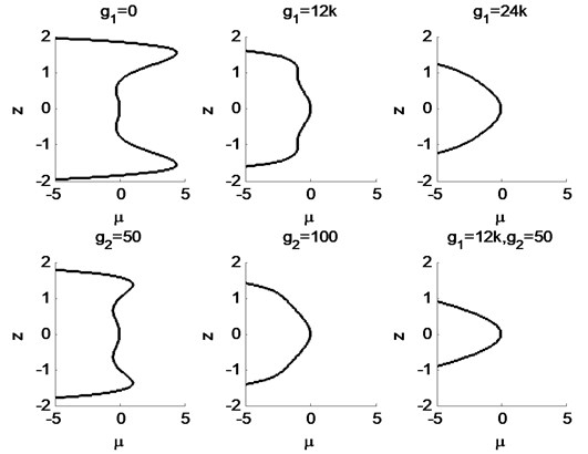
Fig. 11 is the static bifurcation control diagram of the system under the condition of the main resonance. Among them, $g_{1}$ and $g_{2}$ determine the value of $α$ and $β$ . The proper selection of $g_{1}$ and $g_{2}$ value can make the system fall into different regions of the transfer, and ultimately determine the movement of the system. From the simulation results of Fig. 11, we can see that with the change of $g_{1}$ and $g_{2}$ value, the vibration of the system changes from instability to critical stability, and finally reaches a stable motion.

As for exerting the addition force on the system, the utility model can be applied to the hydraulic cylinder of rolling mill, and the vibration of the roller can be controlled by adding a vibration absorber.

6. Conclusions

Considering the effect of horizontal vibration of rolled piece, a coupling vibration model of the roll system is established. By introducing the time delay feedback into the coupling system, a coupled vibration control model of rolling mill is proposed. Then by using the multiple scales method, the amplitude frequency response equation considering the system principal resonance and internal resonance are obtained. Finally, the influence of the feedback gain parameter and time delay on the amplitude frequency characteristic of roll system is studied. At the same time, the jumping phenomenon that avoids the bifurcation of the vibration amplitude of the roll system of the rolling mill is given. Through the analysis of numerical simulation, the main conclusions are obtained as follows:

1) According to the singularity theory, the transition sets and bifurcation diagrams are obtained under the condition of the main resonance and internal resonance. The results show that the stability of the system is different with the change of bifurcation parameters. If the bifurcation parameter is chosen properly, the “jump phenomenon” often appears in the amplitude frequency curve of the system will be reduced or even avoided.

2) By introducing the feedback of displacement and velocity, the control effect of the system is obtained. By adjusting the parameters of feedback gain and time delay, the bifurcation behavior of the roll vibration is effectively suppressed, which greatly improves the ability of the system to resist the disturbance of parameters and external excitation.

References

Fujita N., Kimura Y., Kobayashi K., et al. Dynamic control of lubrication characteristics in high speed tandem cold rolling. Journal of Materials Processing Technology, Vol. 229, 2016, p. 407-416.

Publisher
Kim Y., Kim C. W., Lee S., et al. Dynamic modeling and numerical analysis of a cold rolling mill. International Journal of Precision Engineering and Manufacturing, Vol. 14, Issue 3, 2013, p. 407-413.

Publisher
Brusa E., Lemma L. Numerical and experimental analysis of the dynamic effects in compact cluster mills for cold rolling. Journal of Materials Processing Technology, Vol. 209, Issue 5, 2009, p. 2436-2445.

Publisher
Hu Peihua, Zhao Huyue, Ehmann K. F. Third-octave-mode chatter in rolling. Part 1: Chatter model. Proceedings of the Institution of Mechanical Engineers, Part B: Journal of Engineering Manufacture, Vol. 20, Issue 8, 2006, p. 1267-1277.

Publisher
Hu Peihua, Zhao Huyue, Ehmann K. F. Third-octave-mode chatter in rolling. Part 2: Stability of a single-stand mill. Proceedings of the Institution of Mechanical Engineers, Part B: Journal of Engineering Manufacture, Vol. 220, Issue 8, 2006, p. 1279-1292.

Publisher
Yun I. S., Wilson W. R. D., Ehmann K. F. Chatter in the strip rolling process, Part I: dynamic model of rolling. Journal of Manufacturing Science and Engineering, Vol. 120, Issue 2, 1998, p. 330-336.

Publisher
Yun I. S., Wilson W. R. D., Ehmann K. F. Chatter in the strip rolling process, Part II: dynamic rolling experiments. Journal of Manufacturing Science and Engineering, Vol. 120, Issue 2, 1998, p. 337-342.

Publisher
Fujita N., Kimura Y., Matsubara Y., et al. Lubrication control technology in tandem cold-rolling mills: high-speed rolling by hybrid-lubrication system in tandem cold-rolling mills II. Journal of the JSTP, Vol. 55, Issue 640, 2014, p. 445-450.

Publisher
Yoo S. J. Neural-network-based decentralized fault-tolerant control for a class of nonlinear large-scale systems with unknown time-delayed interaction faults. Journal of the Franklin Institute, Vol. 351, Issue 3, 2014, p. 1615-1629.

Publisher
Yoo S. J. Adaptive fault compensation control for a class of nonlinear systems with unknown time-varying delayed faults. Nonlinear Dynamics, Vol. 70, Issue 1, 2012, p. 55-65.

Publisher
Zhang Y., Yan X., Ling Q. Electromechanical coupling vibration of rolling mill excited by variable frequency harmonic. Advanced Materials Research, Vol. 912, Issue 914, 2014, p. 662-665.

Publisher
Zhang Y., Yan X., Lin Q. Characteristic of torsional vibration of mill main drive excited by electromechanical coupling. Chinese Journal of Mechanical Engineering, Vol. 29, Issue 1, 2016, p. 1-8.

Publisher
Orlowska-Kowalska T., Szabat K. Damping of torsional vibrations in two-mass system using adaptive sliding neuro-fuzzy approach. IEEE Transactions on Industrial Informatics, Vol. 4, Issue 1, 2008, p. 47-57.

Publisher
Fang Y., Wang Z., Xie Y., et al. Sliding mode variable structure control of multi-model switching for rolling mill hydraulic servo position system. Electric Machines and Control, Vol. 14, Issue 5, 2010, p. 91-96.

Search CrossRef
Liu F., Liu B., Liu H., et al. Vertical vibration of strip mill with the piecewise nonlinear constraint arising from hydraulic cylinder. International Journal of Precision Engineering and Manufacturing, Vol. 16, Issue 9, 2015, p. 1891-1898.

Publisher

Cited by

Vibration Energy Coupling Behavior of Rolling Mills under Double Disturbance Conditions

Lidong Wang | Shen Wang | Xingdou Jia | Xiaoling Wang | Xiaoqiang Yan

(2023)

Stability of nonlinear vibrations induced by rolling force in a precise cold mill system

Chaofan Sun | Wu Zhao | Dan Huang | Hongbin Zhang

(2023)

Vibration transmission and energy dissipation of roll controlled by particle damping absorber

Huidong Xu | Ming Wang | Dongping He | Tao Wang

(2023)

Vertical–Horizontal Coupling Vibration of Hot Rolling Mill Rolls under Multi-Piecewise Nonlinear Constraints

Rongrong Peng | Xingzhong Zhang | Peiming Shi

(2021)

Coupled Vibration Behavior of Hot Rolling Mill Rolls under Multinonlinear Effects

Rongrong Peng | Xingzhong Zhang | Peiming Shi

(2020)

About this article

Received

20 April 2017

Accepted

17 July 2017

Published

31 December 2017

SUBJECTS

Vibration generation and control

DOI

https://doi.org/10.21595/jve.2017.18514

Keywords

strip rolling mill

dynamic rolling force

multiple scales method

stability analysis

time delayed feedback

Acknowledgements

This work is supported by the National Natural Science Foundation, China (Grant No. 61673334).

Author Contributions

Zhaolun Liu contributed significantly to date analyses and wrote the manuscript. Jiahao Jiang contributed to the manuscript preparation and programming. Peng Li helped perform the analysis with constructive discussions. Guixiang Pan performed the data analyses. Bin Liu contributed to the conception of the study and revised the manuscript.

This is an open access article distributed under the Creative Commons Attribution License, which permits unrestricted use, distribution, and reproduction in any medium, provided the original work is properly cited.

Previous article in issue Previous Next article in issue Next

Research article

2024 01 21

Study on the effect of rolling mill dynamic stiffness on coupled vibration of hydraulic machine

Lidong Wang, Peng Hou, Shen Wang, Chengzhen Wang, Xiaoqiang Yan, Xiaoling Wang

Research article

2021 08 06

Nonlinear vibration characteristics and time-delayed displacement control of rolling mill under dynamic rolling force

Rongrong Peng

Research article

2017 11 15

Influence of asymmetric structure parameters on rolling mill stability

Jinlei Huang, Yong Zang, Zhiying Gao, Lingqiang Zeng

Research article

2016 12 31

Analytical solution for nonlinear vertical vibration model of mill roll system based on improved complexification averaging method

Yong Zhu, Wan-lu Jiang, Xiang-dong Kong, Hao-nan Wang

Z. Liu, J. Jiang, P. Li, G. Pan, and B. Liu, “Dynamic analysis and control of strip mill vibration under the coupling effect of roll and rolled piece,” Journal of Vibroengineering, Vol. 19, No. 8, pp. 6079–6093, Dec. 2017, https://doi.org/10.21595/jve.2017.18514

Copy Extrica

Copied to clipboard!

TY  - JOUR
DO  - 10.21595/jve.2017.18514
UR  - https://doi.org/10.21595/jve.2017.18514
TI  - Dynamic analysis and control of strip mill vibration under the coupling effect of roll and rolled piece
T2  - Journal of Vibroengineering
AU  - Liu, Zhaolun
AU  - Jiang, Jiahao
AU  - Li, Peng
AU  - Pan, Guixiang
AU  - Liu, Bin
PY  - 2017
DA  - 2017/12/31
PB  - JVE International Ltd.
SP  - 6079-6093
IS  - 8
VL  - 19
SN  - 1392-8716
ER  - 

Copy Ris

Copied to clipboard!

@article{Liu_2017,
	doi = {10.21595/jve.2017.18514},
	url = {https://doi.org/10.21595/jve.2017.18514},
	year = 2017,
	month = {dec},
	publisher = {{JVE} International Ltd.},
	volume = {19},
	number = {8},
	pages = {6079--6093},
	author = {Zhaolun Liu and Jiahao Jiang and Peng Li and Guixiang Pan and Bin Liu},
	title = {Dynamic analysis and control of strip mill vibration under the coupling effect of roll and rolled piece},
	journal = {Journal of Vibroengineering}
}

Copy Bibtex

Copied to clipboard!

[1]Z. Liu, J. Jiang, P. Li, G. Pan, and B. Liu, “Dynamic analysis and control of strip mill vibration under the coupling effect of roll and rolled piece,” Journal of Vibroengineering, vol. 19, no. 8, pp. 6079–6093, Dec. 2017, doi: 10.21595/jve.2017.18514.

Copy IEEE

Copied to clipboard!

Liu, Zhaolun, Jiahao Jiang, Peng Li, Guixiang Pan, and Bin Liu. “Dynamic Analysis and Control of Strip Mill Vibration under the Coupling Effect of Roll and Rolled Piece.” Journal of Vibroengineering 19, no. 8 (December 31, 2017): 6079–93. https://doi.org/10.21595/jve.2017.18514.

Copy Chicago

Copied to clipboard!

Dynamic analysis and control of strip mill vibration under the coupling effect of roll and rolled piece

Abstract

1. Introduction

2. Dynamic formula of rolling force and friction

3. Coupled vibration control model of strip mill

4. Coupling system solution of strip mill based on time delay feedback

4.1. System response in the case of primary resonance

4.2. System response in the case of Internal resonance

5. Characteristic analysis and control of strip mill

5.1. Vibration time domain control of rolling mill system

5.2. Vibration amplitude frequency control of rolling mill system

5.3. Bifurcation stability control of main resonance of rolling mill the roll system

6. Conclusions

References

Cited by

About this article

Related Articles