Abstract
To diagnose rotating machinery fault for imbalanced data, a kind of method based on fast clustering algorithm and decision tree is proposed. Combined with wavelet packet decomposition and isometric mapping (Isomap), sensitive features of different faults can be obtained so the imbalanced fault sample set is constituted. Then the fast clustering algorithm is applied to search core samples from the majority data of the imbalanced fault sample set. Consequently, the balanced fault sample set consisted of the clustered data and the minority data is built. After that, decision tree is trained with the balanced fault sample set to get the fault diagnosis model. Finally, gearbox fault data set and rolling bearing fault data set are used to test the fault diagnosis model. The experiment results show that proposed fault diagnosis model could accurately diagnose the rotating machinery fault for imbalanced data.
1. Introduction
With the rapid progress of modern science and technology, large rotating machinery equipment such as wind turbines, gas turbines and others become more and more complex. Considering the impact of unpredictable factors, failures of the rotating machinery equipment are different to avoid [1-3]. Since these failures would cause serious economic loss. To avoid huge economic loss, accurate and timely fault diagnosis is very significant for the rotating machinery. Recently, novel technologies and algorithms have been widely applied to rotating machinery fault diagnosis [4, 5]. For rotating machinery, types of faults are various while some failures don't happen very often. Herein the fault sample set would be imbalanced. Therefore, it is necessary to develop rotating machinery fault diagnosis technology for imbalanced fault sample set.
Decision tree is a kind of classification algorithm which has been widely applied in fault diagnosis. It adopts the top-down recursive regulation and attribute values are compared in the internal nodes of the decision tree. And conclusions can be got at the leaf nodes [6-8]. Compared with artificial neural network, the classification principle of decision tree is simple and easy to understand. At the same time, the classification model based on decision tree calculates fast. To increase the comprehensibility and usability of the decision tree in the process of establishing the decision tree, the pruning method can be used to prevent the decision tree from being too complicated. Even though pruning decision tree can avoid the over-fitting of the decision tree, the information gain of the decision tree will still be easily affected in the imbalanced training sample set [9-10]. The result of the information gain will still be biased towards those features with more values. Therefore, the pre-processing of the data set is necessary.
Since the cluster algorithm could classify the data according to their similarity, an approach based on fast clustering algorithm is adopted to search the core samples from the majority data of the imbalanced data set. This kind of fast clustering algorithm is proposed by Alex Rodriguez and Alessandro Laio in 2014. The main idea of this clustering algorithm [11-13] is automatically excluding the outliers from the original data set, so it is suitable for extracting the core samples and balance the imbalanced data set.
A kind of method based on fast clustering algorithm and decision tree is proposed to diagnose rotating machinery fault for imbalanced data. The vibration signal of the rotating machinery is decomposed into different frequency bands by wavelet packet decomposition, thus the original features can be got. After that, Isomap is applied to reduce the dimension of original features and obtain sensitive features. The fast clustering algorithm is used to construct the balanced data set. Finally, decision tree is trained to get the fault diagnosis model.
2. Decision tree and fast clustering algorithm
2.1. Fundamentals of decision tree
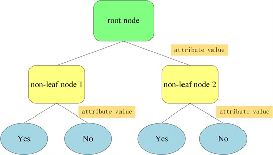
For decision tree, the top-down recursive method is adopted. The attribute values are compared in the internal nodes of the decision tree, and then the branches are developed from the internal nodes according to the different attributes. Finally, the conclusion can be concluded at the leaf nodes. Therefore, how to construct a decision tree with high precision and small scale is the core of the decision tree algorithm. Fig. 1 shows the schematic diagram of the decision tree. In Fig. 1, each non-leaf node represents an attribute of the training samples. The attribute value indicates the value corresponding to the attribute. And leaf nodes represent the sample category attributes.
Fig. 1Schematic diagram of the decision tree
In the process of training the decision tree, it is significant to choose the basis for testing attributes. The information gain is usually used as the basis for the generation of nodes. By selecting the attribute with the highest information gain as the testing attribute of the current node, the mixing level of training samples at this node will be reduced to the lowest. In order to precisely define the information gain, we first define the entropy, a metric that is widely used in information theory.
If the sample set is , and the value of the attribute is , then the entropy of the sample set S is defined as [14, 15]:
where is the proportion of the th attribute value sample set.
Then the information gain can be formed as:
where is the range of the attribute , represents the sample set that the value of the attribute is .
In different candidate attributes, the attribute with the largest information gain is selected as the classification basis of the current decision node. Then the new decision nodes are constantly created, and finally a decision tree to classify the training sample set can be established.
2.2. Pruning decision tree
To avoid the over-fitting and reduce the complexity of the decision tree, it is necessary to prune the decision tree. The pruning decision tree is to delete the most unreliable branches by statistical methods, so the probability of over-fitting can be weakened. Generally, the main pruning methods include pre-pruning and post-pruning [16, 17]. The pre-pruning is usually based on the statistical significance to determine whether the current node needs to divide continuously. It is difficulty to choose a suitable threshold which directly determine the classification degree of the decision tree. Compared with pre-pruning, post-pruning allows the decision tree to grow sufficiently. Then the extra branches would be pruned, so the post-pruning can obtain a more accurate decision tree. The pruning decision tree would consider the coding length of the decision tree. The minimum description length (MDL) principle is adopt to optimize the decision tree. The basic idea is to construct the decision tree with the shortest coding length.
Although pruning the decision tree can avoid the over-fitting of the decision tree, the information gain of the decision tree will still be easily affected in the imbalanced training sample set. The result of the information gain will still be biased towards those features with more values. Therefore, in order to improve the classification performance of decision tree for imbalanced sample set, a fast clustering algorithm is applied to balance the sample set.
2.3. Fast clustering algorithm
A kind of fast clustering algorithm is adopted to balance the original data set. The basic idea of this clustering algorithm is automatically excluding the outliers, so it is suitable for extracting the core samples from the imbalanced data set. The assumptions of the algorithm are that cluster centers are surrounded by neighbors with lower local density. In addition, these cluster centers are at a relatively large distance from any points with a higher local density. The local density can be calculated by Cut-off kernel. With Cut-off kernel, the local density of data point can be formulated as [11, 12]:
where is the distance between data point and data point and is the cut-off distance.
In Eq. (3), the local density represents the number of the data points which are closer to data point compared with . Then the distance can be expressed as:
It is clear that the distance means the minimum distance between the point and the point with higher density, except that the point possesses the highest density. For the point with highest density, we conventionally take:
The local density and distance for each data point can be calculated. Therefore, the weight of clustering center is constructed as:
Obviously, the clustering centers are the points with larger weights. So, the sequence can be constructed as:
where sequence is the index number of local density sorted in descending order. The sequence represents the index number of the point closest to point , while the local density of this point is larger than point .
After that, the non-clustering center points can be categorized as:
where are the labels of the clustering centers.
In the imbalanced data set, the mean local density of each cluster can be calculated. Then the cluster can be divided into core points and halo points by comparing with the mean local density.
Fig. 2“Synthetic point distributions” data set
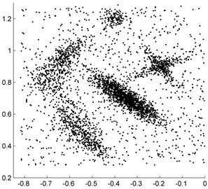
a) Raw data
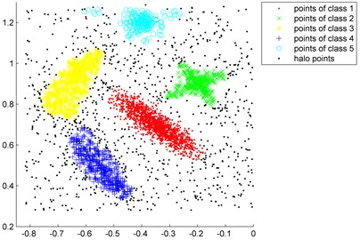
b) Clustered by fast clustering algorithm
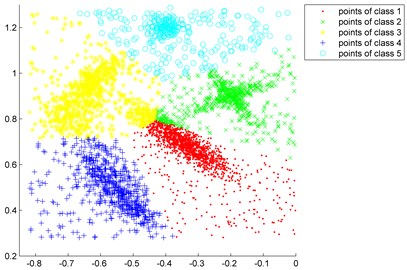
c) Clustered by K-means clustering algorithm
To test the effectiveness of the fast clustering algorithm, the “Synthetic point distributions” data set is applied [11]. The distribution of the “Synthetic point distributions” data set are shown in Fig. 2. From Fig. 2(b), we can see that the core points of five class data are all correctly selected from the raw “Synthetic point distributions” data set. Fig. 2(c) shows the clustering result of the K-means clustering algorithm, it is clear that the raw data are approximately divided into five categories while the noise points are not eliminated. This illustrates that the fast clustering algorithm can be well applied to extract the core samples from the imbalanced data set.
3. Rotating machinery fault diagnosis for imbalanced data
3.1. Feature extraction and dimension reduction
The vibration signal of the rotating machinery usually consists of a series of complex components. To decompose the vibration signal into different frequency bands. The wavelet packet decomposition is applied. The output of the th layer can be defined as during the process of decomposing the vibration signal, where represents the time serial number. The decomposition formulas are as follows [18-20]:
where and are the outputs of the ()th layer.
The wavelet “coiflet” is adopted. The condition corresponds to a “coiflet” of order is defined as:
where Eq. (12) is the condition that the vanishing moment of scaling function equals to zero. And Eq. (13) is the condition that the vanishing moment of wavelet equals to zero.
Meanwhile:
where are the coefficients.
After decomposing the vibration signal of the rotating machine into different frequency bands, the energy of each sub-frequency band is calculated. Then the original features can be constructed. To reduce the dimension of the original features, Isomap is applied to obtain the sensitive features. The main calculating stages of the Isomap are as follows [21-22]:
(1) Neighborhood graph is constructed. For example, the original data set are . If is one of the nearest neighbors of , might contain the edge when ;
(2) Euclidean length is calculated. The shortest paths should be calculated for all pairs of data points;
(3) Embedded Data. With the method of multidimensional scaling (MDS), the new embedment of the data in Euclidean space can be searched.
3.2. Balanced data set and fault diagnosis model
The rotating machinery fault sample set usually contains various fault types. Since some fault types are frequent faults while others are accidental, ordinarily the rotating machinery fault sample set is an imbalanced data set. For each fault sample, a number of sensitive features can be obtained by Isomap. Then the distance between two fault samples can be formulated as:
where and are the sensitive features of the th fault sample and the th fault sample. is the weight of the th sensitive feature. represents the number of sensitive features for each fault sample.
Fig. 3Flowchart of building fault diagnosis model
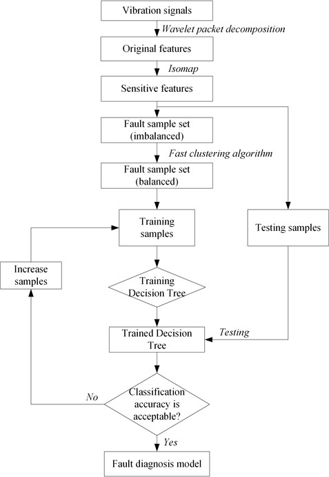
After calculating the distance , the local density and the distance can be got based on Eqs. (3-6). Then referencing the Eq. (7), the weight of each fault sample can be obtained. Considering the number of samples of the minority fault type, the same number of samples with higher weight are selected from the majority type. Thus, the balanced fault sample set is constructed by whole samples from minority fault type and selected samples from the majority type. Eventually, the decision tree classification algorithm is applied to study the balanced fault sample set, so the fault diagnosis model can be obtained. Fig. 3 shows the flowchart of building fault diagnosis model.
It is clear that the balanced sample set are used to train the decision tree, while the testing samples are responsible for testing the classification accuracy of the trained decision tree. The trained decision tree would not be adopted until the classification accuracy is acceptable. Thus, the trained decision tree can be recognized as the fault diagnosis model.
4. The experiment results
Gearbox and rolling bearing are two kinds of common rotating machinery components. Therefore, fault data sets of gearbox and rolling bearing are both adopted to test the validity of the proposed fault diagnosis model.
4.1. Gearbox fault diagnosis
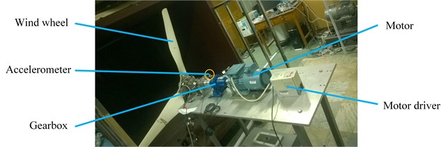
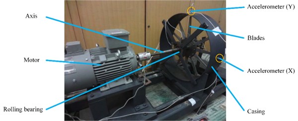
The gearbox failure simulation test bed is shown in Fig. 4. The main components include gearbox, motor, motor driver, wind wheel and accelerometer. The motor is responsible for driving the gearbox at different rotating speeds. The function of the wind wheel is as a load. An accelerometer is installed on the top of the gearbox and used for acquiring the vibration signal. The type of the tested gearbox is single-stage planetary transmission. Meanwhile the number of the planetary gear teeth is 20. In the testing, two kinds of planetary gear failures are adopted: half fracture and full fracture. To simulate the real working condition, the rotating speed is also considered in the testing. As is shown in Table 1, the rotating speed includes 157 r/min, 237 r/min and 317 r/min. The sampling frequency of the data acquisition is 25 kHz while the sampling time for each sample is 0.4 seconds. Thus, there are 10000 data points in each sample.
Table 1Testing for gearbox
Planetary gear | Rotating speed (r/min) | |
Testing 1 | Normal | 157/237/317 |
Testing 2 | Half fracture | 157/237/317 |
Testing 3 | Full fracture | 157/237/317 |
Fig. 4Gearbox failure simulation test bed
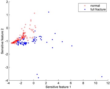
With the method of wavelet packet decomposition, the gearbox vibration signal can be decomposed into different frequency bands. Then the energy of each frequency band is calculated, so the original features can be obtained. To get the sensitive features, Isomap dimension reduction algorithm is adopted. Thus, sensitive feature 1, sensitive feature 2 are selected. Fig. 5 show the distributions of sensitive features. In order to test the effectiveness of Isomap, calculating result by principal component analysis (PCA) is also shown in Fig. 5(a). From Fig. 5(a), it can be seen that the distribution areas of normal gear, half fracture and full fracture are mixed. In Fig. 5(b), the aliasing region only exists between normal gear and full fracture. Since the aliasing region would lead to the misjudgment between different failures. Therefore, testing data from the normal gear and full fracture are used to construct an imbalanced data set to test the classification effect of the proposed fault diagnosis model.
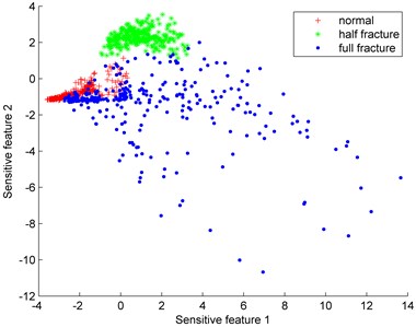
Fig. 6 show the distributions of the imbalanced data set under different proportions (normal: full fracture). Since the normal gear data is much easier to obtain than the full fracture data, the normal gear is defined as the majority class while the full fracture is the minority class. The number of the normal gear is 150 and the number of the full fracture data varies from 30 to 80.
Fig. 5Distributions of sensitive features
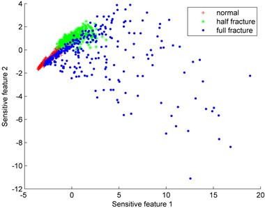
a) PCA
b) Isomap
The imbalanced data sets shown in Fig. 6 are adopted as the training samples. The testing samples are composed of 300 samples. 150 samples are from normal gear data while another 150 samples are from full failure data. Meanwhile, decision tree models are also trained for comparing with the proposed fault diagnosis model. Table 2 and Fig. 7 show the classification accuracy comparisons between proposed fault diagnosis model and other methods. We can see that pruning has no effect on the improvement of decision tree classification accuracy for the imbalanced data set. To show the advantage of the fast clustering algorithm for extracting the core samples, K-means clustering algorithm is also adopted for comparing. Since K-means clustering algorithm is a similarity measure method based on Euclidean distance, so the algorithm is suitable for clusters of spherical shapes. Thus, the core samples extracted by K-means clustering algorithm are mostly gathered together. Therefore, the decision tree trained by these gathered core samples is not suitable to the entire imbalance data set. It is clear that the classification accuracy of the K-means clustering algorithm is less than other methods in Table 2.
Table 2Classification accuracy comparisons between fault diagnosis model and other methods
Proportion of the data set | 150:30 | 150:40 | 150:50 | 150:60 | 150:70 | 150:80 |
Fault diagnosis model | 92.33 % | 92.00 % | 92.00 % | 93.00 % | 92.67 % | 92.33 % |
Decision tree before pruning | 87.67 % | 88.33 % | 90.00 % | 90.00 % | 90.00 % | 90.67 % |
Decision tree after pruning | 86.00 % | 88.33 % | 89.33 % | 89.00 % | 89.67 % | 89.67 % |
K-means and decision tree | 81.33 % | 81.33 % | 84.00 % | 84.33 % | 79.00 % | 77.67 % |
Table 3Training time comparisons between fault diagnosis model and other methods
Proportion of the data set | 150:30 | 150:40 | 150:50 | 150:60 | 150:70 | 150:80 |
Fault diagnosis model | 0.9048 s | 0.9375 s | 0.9450 s | 0.9559 s | 0.9588 s | 0.9806 s |
Decision tree before pruning | 0.1886 s | 0.1904 s | 0.1914 s | 0.1924 s | 0.1927 s | 0.1935 s |
Decision tree after pruning | 0.5883 s | 0.6088 s | 0.6227 s | 0.6282 s | 0.6364 s | 0.6451 s |
K-means and decision tree | 0.6326 s | 0.6655 s | 0.6856 s | 0.6910 s | 0.6949 s | 0.7149 s |
The classification accuracies of the fault diagnosis model in different data sets are all more than 92 %. It is obvious that the fault diagnosis model has achieved better classification results than other methods.
Table 3 show the training time comparisons between fault diagnosis model and other methods. In this paper, the hardware environment is as follows: the processor is Intel Core i7-4600U. The memory is 8 GB and the operating system is Windows8. Meanwhile, the software environment is MATLAB R2013b. As can be seen from Table 3, the training time of four methods is less than 1 second. It would take time for clustering the data, so the training time of “fault diagnosis model” and “K-means and decision tree” is longer than other two methods. To sum up, the training time of the fault diagnosis model is acceptable since the fault diagnosis model has achieved better classification results than other methods.
Fig. 6Distributions of the imbalanced data set under different proportions (normal: full fracture)
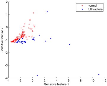
a) 150:30
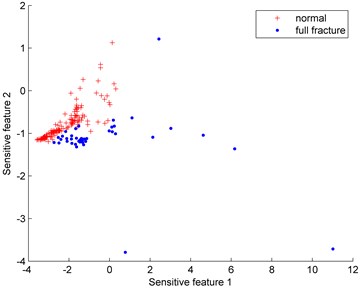
b) 150:40
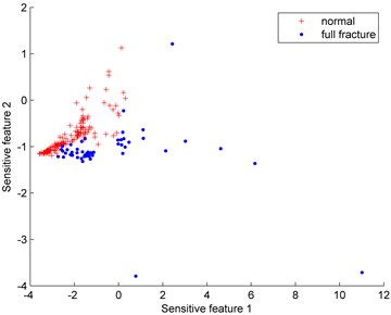
c) 150:50
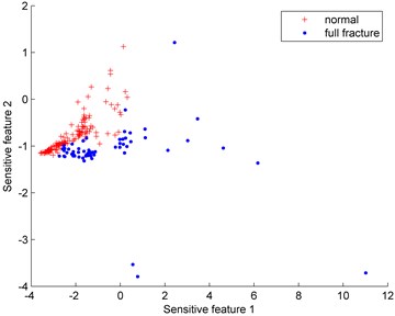
d) 150:60
e) 150:70
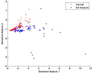
f) 150:80
4.2. Rolling bearing fault diagnosis based on casing vibration
In the case of gearbox fault diagnosis, the gearbox failure data set is applied to test the proposed fault diagnosis model when the data set only includes two kinds of failures. To test the model’s classification performance when the imbalanced data set includes multiple failures, the rolling bearing failure data set is adopted.
Fig. 8 shows the structure of the rolling bearing failure simulation test bed. As is shown in Fig. 8, one end of the axis is connected with a motor, while the other end is fit together with several blades and the testing rolling bearing. A casing is installed around the blades. Two accelerometers are fixed on the surface of the casing at a 90-degree angle. The motor which is responsible for driving blades and two accelerometers are used for monitoring the vibration of the rolling bearing. The rotating speed is 1800 rpm while the sampling frequency of the data acquisition system is 16 kHz. The sampling time for each sample is 0.2 seconds, and there are 3200 data points in each sample. The rolling bearing failure data set is made up of four kinds of types, such as normal, rolling element failure, inner race failure and outer race failure.
Fig. 7Classification accuracy comparisons among fault diagnosis model and other methods
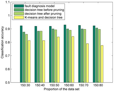
Fig. 8Rolling bearing failure simulation test bed
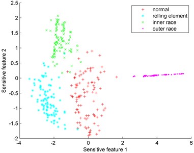
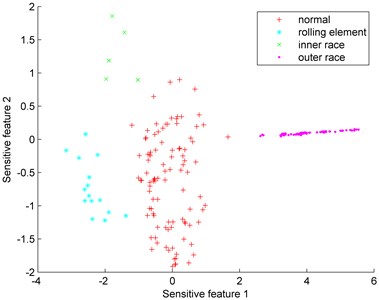
After feature extraction and dimension reduction, the distributions of sensitive features of four types can be obtained and shown in Fig. 9. In Fig. 9(a), the number of samples is 400 (100 samples for each type). It is clear that rolling element type and outer race type have been distinguished. The aliasing region only exists between normal type and inner race type. Fig. 9(b) shows the distribution of the imbalanced data set. The composition of the imbalanced rolling bearing data set is introduced in Table 4. The rolling element failure type and inner race failure are treated as minority class to test the proposed fault diagnosis model.
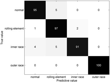
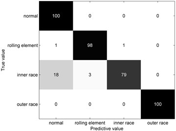
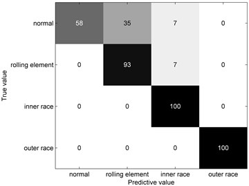
The imbalanced rolling bearing data set is applied to train the fault diagnosis model. Then, the testing samples consist of 400 samples (100 samples for each type) are founded. Meanwhile, the decision tree model is also trained and tested for comparing. Fig. 10 show the confusion matrix comparisons. From Fig. 10(b), it is obvious that the decision tree is confused with inner race type and normal type. This illustrates the decision tree is easily affected by the aliasing region especially in the imbalanced data set. From Fig. 10(c), it is obvious that the trained decision tree is confused with normal type and rolling element type. This shows the core samples extracted by K-means clustering algorithm are mostly gathered together for normal type and rolling element type. By contrast, the fault diagnosis model can distinguish four types from the testing sample very well, which proves the validity of the proposed approach.
The training time of “fault diagnosis model”, “decision tree” and “K-means and decision tree” were 1.5804 seconds, 0.1857 seconds, and 0.3044 seconds respectively.
Fig. 9Distributions of sensitive features
a) Balanced data set
b) Imbalanced data set
Fig. 10Confusion matrix comparisons
a) Fault diagnosis model
b) Decision tree
c) K-means and decision tree
Table 4Composition of the imbalanced rolling bearing data set
Mode | Processing method | Fault size (width×depth) (mm) | The number of samples |
Normal | – | – | 100 |
Rolling element failure | Line cutting | 0.3×1 | 15 |
Inner race failure | Line cutting | 0.3×0.5 | 5 |
Outer race failure | Line cutting | 0.3×0.5 | 100 |
5. Conclusions
The fault diagnosis model based on fast clustering algorithm and decision tree is proposed in this paper. The experiment results illustrate that our proposed fault diagnosis model achieves better classification performance than the decision tree models. Some conclusions can be obtained as follows:
1) For rolling bearing, accelerometers installed on the surface of the casing can be used to monitor the vibration of the rolling bearing while the acceleration signals can be applied to diagnose the faults;
2) Since some failure samples of rotating machinery are not easy to obtain, the failure data set is likely to be an imbalanced data set. This paper proposed an approach based on fast clustering algorithm and decision tree for rotating machinery diagnosis. The fast clustering algorithm is applied for extracting core samples from the original data set, so the balance data set can be established. Then decision tree is trained and tested with the data clustered by fast clustering algorithm, so the fault diagnosis model for imbalanced data can be obtained. To show the advantage of the fast clustering algorithm for extracting the core samples, K-means clustering algorithm is also adopted for comparing. The experiment results show that the fault diagnosis model demonstrates a very good classification performance both for gearbox data set and rolling bearing data set. Meanwhile, the training time of the fault diagnosis model is also acceptable. Thus, proposed fault diagnosis model is adapted to rotating machinery fault diagnosis for imbalanced data.
References
-
Jay J., Wu F. J., Zhao W. Y., et al. Prognostics and health management design for rotary machinery systems – reviews, methodology and applications. Mechanical Systems and Signal Processing, Vol. 42, Issues 1-2, 2014, p. 314-334.
-
Liu C., Jiang D. X. Crack modeling of rotating blades with cracked hexahedral finite element method. Mechanical Systems and Signal Processing, Vol. 46, Issue 2, 2014, p. 406-423.
-
Yan R. Q., Gao R. X., Chen X. F. Wavelets for fault diagnosis of rotary machines: a review with applications. Signal Processing, Vol. 96, 2014, p. 1-15.
-
Lei Y. G., Lin J., He Z. J., et al. A review on empirical mode decomposition in fault diagnosis of rotating machinery. Mechanical Systems and Signal Processing, Vol. 35, Issues 1-2, 2013, p. 108-126.
-
Liu C., Jiang D. X., Yang W. G. Global geometric similarity scheme for feature selection in fault diagnosis. Expert Systems with Applications, Vol. 41, Issue 8, 2014, p. 3585-3595.
-
Pal A., Thorp J. S., Khan T., et al. Classification trees for complex synchrophasor data. Electric Power Components and Systems, Vol. 41, Issue 14, 2013, p. 1381-1396.
-
Kang M., Kim M., Lee J. H. Analysis of rigid pavement distresses on interstate highway using decision tree algorithms. KSCE Journal of Civil Engineering, Vol. 14, Issue 2, 2010, p. 123-130.
-
Akkas E., Akin L., Cubukcu H. E., et al. Application of decision tree algorithm for classification and identification of natural minerals using SEM-EDS. Computers and Geosciences, Vol. 80, 2015, p. 38-48.
-
Yi W. G., Lu M. Y., Liu Z. Multi-valued attribute and multi-labeled data decision tree algorithm. International Journal of Machine Learning and Cybernetics, Vol. 2, Issue 2, 2011, p. 67-74.
-
Amarnath M., Sugumaran V., Kumar H. Exploiting sound signals for fault diagnosis of bearings using decision tree. Measurement, Vol. 46, Issue 3, 2013, p. 1250-1256.
-
Rodriguez A., Laio A. Clustering by fast search and find of density peaks. Science, Vol. 344, Issue 6191, 2014, p. 1492-1496.
-
Mehmood R., Zhang G. Z., Bie R. F., et al. Clustering by fast search and find of density peaks via heat diffusion. Neurocomputing, Vol. 208, 2016, p. 210-217.
-
Mehmood R., Bie R. F., Jiao L. B., et al. Adaptive cutoff distance: Clustering by fast search and find of density peaks. Journal of Intelligent and Fuzzy Systems, Vol. 31, Issue 5, 2016, p. 2619-2628.
-
Yasami Y., Mozaffari S. P. A novel unsupervised classification approach for network anomaly detection by k-Means clustering and ID3 decision tree learning methods. Journal of Supercomputing, Vol. 53, Issue 1, 2010, p. 231-245.
-
Jin C. X., Li F. C., Li Y. A generalized fuzzy ID3 algorithm using generalized information entropy. Knowledge-Based Systems, Vol. 64, 2014, p. 13-21.
-
Purdila V., Pentiuc S. G. Fast decision tree algorithm. Advances in Electrical and Computer Engineering, Vol. 14, Issue 1, 2014, p. 65-68.
-
Luo L. K., Zhang X. D., Peng H., et al. A new pruning method for decision tree based on structural risk of leaf node. Neural Computing and Applications, Vol. 22, 2013, p. 17-26.
-
Pan Y. N., Chen J., Li X. L. Bearing performance degradation assessment based on lifting wavelet packet decomposition and fuzzy c-means. Mechanical Systems and Signal Processing, Vol. 24, Issue 2, 2010, p. 559-566.
-
AI-Badour F., Sunar M., Cheded L. Vibration analysis of rotating machinery using time-frequency analysis and wavelet techniques. Mechanical Systems and Signal Processing, Vol. 25, Issue 6, 2011, p. 2083-2101.
-
Bin G. F., Gao J. J., Dhillon B. S. Early fault diagnosis of rotating machinery based on wavelet packets-empirical mode decomposition feature extraction and neural network. Mechanical Systems and Signal Processing, Vol. 27, 2012, p. 696-711.
-
Zhao X. M., Zhang S. Q. Facial expression recognition based on local binary patterns and kernel discriminant Isomap. Sensors, Vol. 11, Issue 10, 2011, p. 9573-9588.
-
Thnenbaum J. B., de Silva V., Langford J. C. A global geometric framework for nonlinear dimensionality reduction. Science, Vol. 290, Issue 5500, 2000, p. 2319-2322.
Cited by
About this article

The research is supported by National Natural Science Fund of China (11572167). The authors are also grateful to the anonymous reviewers for their worthy comments.
