Abstract
With the development of concepts of industry 4.0, condition monitoring techniques are changing. Large amounts of generated data require diagnostic procedures to be automated, which drives the need for new and better methods of autonomous interpretations of vibration condition monitoring data. However, if new methods are to be operational, they need to be verified under real industrial conditions and compared with well-established expert-based diagnostic techniques. This article introduces the novel algorithm of data preprocessing for the nearest-neighbor-based anomaly detection. This approach is validated on real industrial machinery in a series of case studies. The population of over-hung centrifugal fans, employed in the same industrial process, were monitored continuously according to the proposed methodology for an extended time period. Piezoceramic accelerometers were used to register time-domain vibration data. The data were processed to extract several signal features to serve as inputs to the anomaly detection algorithm. The novel solution is compared to the well-established condition monitoring approach. Presented data include not only the intact state of machinery but also a machine breakdown case and serious deterioration of the machine condition. The influence of maintenance work is also presented in the article. Authors show the data-driven approach to condition monitoring, which can be used as one of many predictive maintenance techniques.
1. Introduction
The fourth industrial revolution (also known as industry 4.0) influences condition monitoring (CM) techniques more and more nowadays [1-3]. Cyclic vibration measurements on rotating machines provide a basis for maintenance strategies in plants. Those, in case of vibration measurements, are mostly based on the comparison of collected data to ISO standards. This approach can be enhanced by the usage of machine learning (ML) algorithms like anomaly detection (AD) [4]. Especially on-line monitoring systems with electronic edge devices, collecting measurements continuously in maintenance applications, need solutions from fields of big data and machine learning.
The growing trend of usage of electronic devices on a wide scale in CM has been triggered by the rapid growth of cloud services and concepts of the Industrial Internet of Things (IIoT), which enables management and analytics of CM data on a big scale. Once an estimate of a measured signal is sent to a database (local or remote), several types of analyses can be performed [5]. In the case of vibration measurements acquired for rotating machinery monitoring, the simplest of these employ a comparison of the statistics of the measured signals with warning and alert thresholds provided by international standards [6]. Although this approach neither provides a meaningful description of the faults developed in the structure nor is sensitive enough to detect damage at an early stage of its growth, due to its simplicity, it is broadly employed in the majority of industrial condition monitoring systems.
In cases when historical data for the specific machine are available, the process of setting thresholds can be improved. Information about machine states in the past can be used to customize the existing thresholds proving the method to be more sensitive. This type of fault detections is presented in the literature either in the form of trend analysis - when vibration signal statistics are plotted against time for the whole monitoring history of the specific machine; or in the multidimensional anomaly or novelty detection - where newly acquired data are compared against a historical dataset to assess whether it exhibits any unexpected properties, which could be treated as a premise of damage. The latter of the approaches is usually deemed more sensitive to small damage, yet it is also more difficult in the configuration.
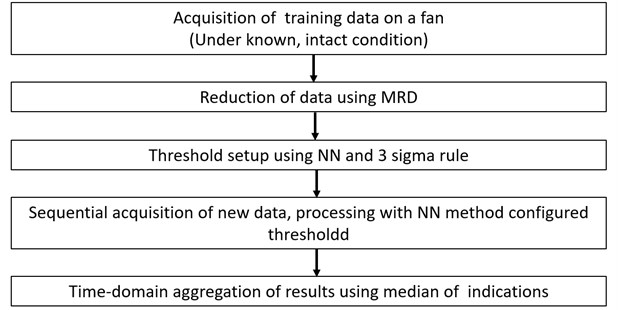
Three significant issues limit the practical application of anomaly detection systems. The first of them is the challenge of proper selection of warning thresholds for the system – if no information about the possible faults is present prior to the system configuration. The second one requires handling of large amounts of data. Finally, the third one deals with the non-uniform distribution of data into clusters, which hinders the operation of many typical anomaly detection algorithms. In order to solve these issues, this study presents the new algorithm for rotating machinery monitoring based on the identification of the most representative dataset (MRD) inspired by the optimal baseline reduction algorithm for the guided-wave-based monitoring [7]. The identified set is used as a source of data for the nearest-neighbor algorithm [8, 9]. The approach is validated using a large set of practical, industrial data acquired for a population of centrifugal fans. Four case studies are performed. The insight provided by the anomaly detection (AD) approach is compared with well-established classical diagnostic techniques [10] and the feedback from the maintenance crew. The proposed approach allows for a significant reduction of stored data, autonomous selection of warning thresholds, and is insensitive to non-uniform distribution of data into clusters.
The organization of the paper is as follows: in Section 2, an anomaly detection algorithm based on the nearest-neighbor method is explained. The algorithm for the reduction of the full dataset to MRD is also described in this Section. Section 3 presents the data acquisition setup, industrial background, and case studies. Finally, Section 4 summarizes and concludes the paper.
2. Anomaly detection algorithm
2.1. The nearest-neighbor (NN) method
An anomaly or novelty is a deviation from a well-defined normal state. In general, anomaly detection requires a collection of normal data, that is: data representing an intact state of the machine, preferably acquired under all possible operational conditions. These data are then used to define a normal region in feature space – with which all of the future measurements should be compared. Samples that would not fall into this region would be considered as anomalies.
An anomaly in the condition monitoring does not necessarily have to be an indication of damage. However, it is a sign that something new is happening to the machine, and it requires a maintenance decision: usually either to stop the machine for maintenance, perform a detailed diagnostic on-line or to continue operations marking the new unknown samples as normal ones. The latter case is often employed when the cause for abnormal data is known, e.g. when a new operational state was deliberately introduced to the system. An advantage of using the anomaly detection lies in a variety of features that can be included simultaneously in the anomaly computation. Therefore, an anomaly may be found not only in values of separate features but also in their mutual relationship. Although the method is designed to operate using only data of the intact state, its main advantage is also its drawback, as it is often difficult to provide an interpretation of the AD system output. In other words, a detected anomaly might represent a near-catastrophic state as well as a slightly deteriorated one.
A novelty detection is broadly employed not only in CM but also in other fields [11-14]. Good reviews of anomaly detection methods were provided by [15] and [16, 17]. In general, the methods can be divided into several categories according to the approach to the normal region definition. In the hereby paper, a method from the distance-based category is used. The distance-based methods are built on the idea that distances between new and known samples in feature space are good indicators of how typical or novel the sample is. There are many methods incorporating this principle (e.g. [18-22]).
In this study the nearest-neighbor method is used. It is arguably one of the simplest approaches in ND, and definitely one of the easiest to implement and understand. Its main disadvantages lie in poor scaling to high-dimensional spaces and poor behavior under non-uniform data distribution. Its main advantage is its straightforward configuration: the method has just one meta-parameter to set up and thus does not require a difficult optimization step, and due to that, it is often preferred in industrial conditions instead of other more advanced and more capable methods. The principle of its operation is depicted in Fig. 1.
Fig. 1Nearest-neighbor anomaly detection principle
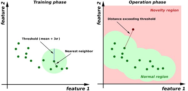
Prior to the operational stage, distances to the closest neighbors of each -th data sample in -element of a normal class are calculated. These distances are then used to set up a threshold – usually equal to the mean of all closest distances plus three times its standard deviation. For each new data sample, a distance to the nearest neighbor belonging to the normal class is calculated. If it is smaller than the threshold, that is if the sample is classified as normal. Otherwise, it is considered an anomaly. The rationale behind such a threshold choice is as follows: if data fall into the Gaussian distribution, the 3σ-threshold provides a correct classification for 99.9 % of normal data samples.
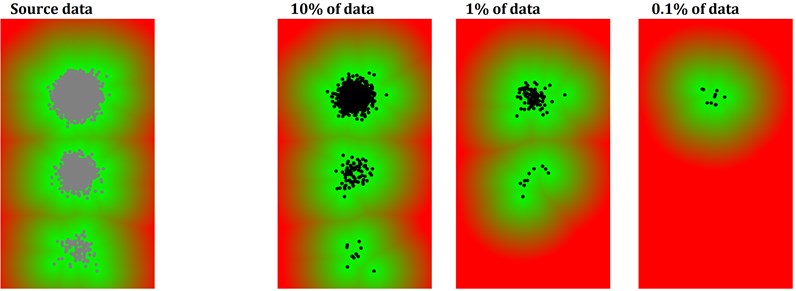
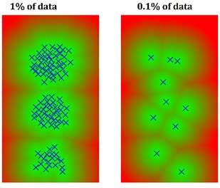
In practical situations, however, the distribution is rarely Gaussian, as usually the normal region is defined by more than one cluster of data. What is more, clusters usually drift through the feature space due to variations of environmental and operational conditions as well as due to an accumulation of structural wear. Since any change in the data distribution might trigger the novelty detection, thresholds need to be set up manually to avoid false-positive indications. What is more, the algorithm requires all the normal samples to be stored in its memory – which becomes a problem if the dataset is either very large from the very beginning or if new data are acquired continuously over an extended time. The typical solution of this problem is reducing the amount of data by taking into consideration only a randomly selected subset of the whole data available. Such an approach, in turn, causes another problem: practical data are often organized in clusters that vary in size by several orders of magnitude. For instance, data representing a normal operation of rotating machinery with its nominal speed may be represented by 99.9 % of the available samples, while the remaining 0.1 % might encompass the run-up or run-down of the machinery. In such case, the reduction of data would likely result in preserving only the nominal-speed-related cluster. AD performed on such a set would yield false alarms every time the machine is stopped. An illustration of this issue is provided in Fig. 2. An artificial dataset is generated randomly in such way that three clusters of data are generated. Clusters contain 10000, 1000, and 100 data samples, respectively. Next, three stages of data reduction are performed by a random selection of 10 %, 1 %, and 0.1 % of data samples. The obtained results do not reflect initial cluster shapes – with less dense clusters disappearing from the distribution entirely. Consequently, any distance-based novelty detection algorithm trained on the reduced dataset would generate false alarms for all the data samples included in the erased clusters.
Fig. 2A multi-cluster normal data set and cluster erased phenomenon due to a random selection of a subset of data. Background color refers to the distance from the nearest sample on the basis of which the distance-based anomaly detection would operate in
2.2. The most representative dataset (MRD)
In order to solve the issue, the authors propose a reduction method for the normal data that preserve borders of clusters by the selection of samples, which are the most representative for the given case. The idea of the algorithm is based on the approach used for compensation of the temperature influence in Lamb-wave-based monitoring – in which a set of most representative baselines was found to cover all typical temperature-induced changes in the received Lamb wave signals [8]. A scheme in Fig. 3 presents a general flow of data in the algorithm.
Fig. 3The flow of data in the algorithm
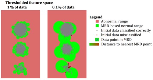
The procedure starts with the selection of a random sample from the normal region. Then, the sample is stored in the MRD. For each iteration of the algorithm, all the samples are compared against all data already included in the MRD. The sample for which distance to the nearest neighbor from the MRD is the biggest, is added to the MRD. The procedure continues until the desired amount of samples in the MRD is reached. The scheme of the -th iteration of the loop is presented in Fig. 4. The result of the algorithm for the same multi-cluster dataset, as presented in Section 2.1, is provided in Fig. 5. It is worth to note that small data clusters are represented as single points in the MRD. Therefore, the spatial density of the MRD remains dependent mostly on the dimensionality of the data and not on the fact of whether they are arranged into one or many clusters. The small clusters do not get discarded during data reduction. Another interesting feature of the algorithm is that if there are many clusters of data in close proximity – which might indicate that data are acquired under many different operational conditions, the algorithm tends to merge them together – which provides a protection from an unexpected cluster drift or slightly changed operational conditions. The threshold for the NN algorithm can be derived straightforwardly from the MRD dataset – using the threshold. Since the MRD already covers data that are the most representative for a given scenario, the threshold is usually much more robust and allows the method to be operational without a manual fine-tuning of the 3 based choice. In the example provided in Fig. 5 this choice allows for 100 % efficiency in the case of 100x data reduction and only for 17 misclassified samples (0.15 % of the whole dataset) in the case of 1000x data reduction. The suitability for handling large amounts of data makes this algorithm an interesting alternative for all other distance-based methods.
Fig. 4The n-th iteration of the MRD selection algorithm. There are already n samples stored in the MRD. For all N-k remaining samples, a minimum dmin, of all the k closest distances, is calculated. A maximum dmin,max of all the N-k minimal distances is calculated, and the corresponding sample is stored in the MRD
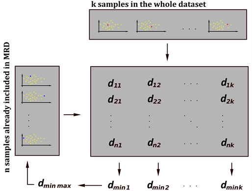
Fig. 5The result of the operation of the MRD selection algorithm a) and normal regions set up on the basis of 3σ rule b) by the threshold distance to nearest MRD point. MRD calculated based on 10 % of data samples is omitted due to clarity of the display
a)
b)
2.3. Time-domain results aggregation
Most of the data acquired under real industrial conditions contain outliers, which are caused by transient changes in external conditions or other environmental factors that cannot be identified or monitored. Despite this fact, the system is not allowed to generate large numbers of false alarms as each of them should be investigated by the qualified staff. On the other hand, diagnostic information that can be derived from acquired signals usually remains similar over many consecutive periods of signal acquisitions. Therefore, to increase the reliability of the system and reduce the number of false alarms, a time-domain aggregation of the obtained diagnose was performed. For each week of monitoring, the median AD indication was calculated. These values served as a final damage index and were displayed for the maintenance crew during the whole monitoring period.
3. Case studies
Many different features can be calculated from raw vibration signals. Some of them are general, some designed for a detection of particular faults [23-26], some require advanced pre-processing of the signals, including envelope [27] analysis, spectral kurtosis calculation [28], cyclo-stationary analysis [29], wavelets [30] or others [31-33]. In this study, however, the illustration of the method is based on probably the simplest - yet the most popular - features listed in Table 1. The rationale behind this choice was to keep the method as general as possible and to avoid tuning it for detection of particular defects without an apriori knowledge of the expected faults since it might bias the research. The four selected features are used as inputs to the NN algorithm (i.e. distances are calculated in four-dimensional feature space). The purpose of this approach is also to give a tool for the phase of condition monitoring which is the fault detection. It is not for localization, classification, assessment or prediction (see [34]). So, in other words, the purpose is to present the novelty detection algorithm which can be a first notification in the real work system of changes that occur at the machine. The list of features can be extended, what would be a very interesting aspect of performing further analyses within this field.
Table 1Features used in the anomaly detection analysis. A is an acceleration feature where yi is a sample of an acceleration signal. V is a velocity feature where xi is a sample in velocity waveform integrated from acceleration time waveform, n refers to signal length
Feature | Formula |
Acceleration RMS | |
Acceleration kurtosis | |
Acceleration peak to peak (pk-pk) | |
Velocity RMS |
Each feature selected for the anomaly detection has its own interpretation in the condition monitoring practice and can be used separately to trend and analyze different kinds of fault conditions present in the machine. The acceleration RMS (Root Mean Square) represents the energy of a raw signal that amplifies high frequencies, which are appropriate to investigate e.g. bearing problems. Kurtosis reflects a peakiness of a signal and allows for a detection of impulses. Peak-to-peak is a feature that amplifies variations of an amplitude. The velocity RMS represents frequency range, which is sensitive to basic rotor dynamics faults like imbalance, misalignment, bearing frequencies, etc. Time domain features presented in the article are calculated from 5-second long acceleration time waveforms.
All presented case studies follow a similar pattern: the section presenting AD analysis of the monitored periods is followed by in-depth analysis of signals using a spectrum-based standard diagnostic procedure. The feedback from the maintenance crew is also discussed in each case study. All four represent performance of the anomaly detection algorithm in different real industrial situations. Four cases are to show the wide variety of situations which can occur in the monitoring of centrifugal over-hung fans, and the reaction of the algorithm for those. Two of the most problematic and often occurring defects (according to descriptions of maintenance crew), at the mentioned over-hung fans are described in the article (unbalance and rolling element bearing defect). The performance of the algorithm is in both cases very promising. Only those two situations show the usability and practicability of this algorithm. The intact state monitoring shows the behavior of an algorithm when none abnormal situation occurs. The simulation approach shows that interpretation of the results must be always done because the detected anomaly does not necessary mean a deterioration of the machine. Presented case studies show a wide spectrum of possible applications for the described algorithm and its applicability as the first detection of changes in the machine.
Results are aggregated into weeks. For the sake of simplicity, only the RMS velocity and acceleration peak-to-peak are presented in figures.
The AD indications and diagnostic features are presented in the form of box plots. The box extends from Q1 to Q3 quartile values of the data with a line at the median Q2. The position of the whiskers is set to 1.5∙IQR (IQR – inter-quartile range). Outlier points are indicated past the end of the whiskers. This way of presenting the data gives also basic statistical information about the data range, outliers, variance, etc. Presented data constitute not a single point but an aggregation of all measured data points in a week, so this covers also - to some extent - the topic of the research uncertainty.
3.1. Data source
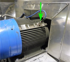
The data presented in the paper are acquired with an on-line monitoring system installed on a population of over-hung centrifugal fans participating in the same manufacturing process. Three of them are analyzed (fan #1, #2, and #3). Machines stand next to each other, indoors, in a plant. Each fan contains a 12 blade impeller being driven by a two-pole pairs induction motor. Each motor shaft is directly connected to a fan rotor. The shaft and impeller are supported only on the motor NDE (Not Drive End) and DE (Drive End) rolling element bearings placed inside the motor. The motor itself is supported on a metal frame vibro-isolated from the ground. Fans operate with a nominal speed of 1465 RPMs. Motors are powered from a supply line of 50 Hz frequency. Fans work 24 hours a day and are stopped only for maintenance works or due to a breakdown. For the sake of meaningful comparison between the monitored fans, sensors were placed at machines in analogous places. Vibration signals are collected with a sampling frequency of 31250 Hz. Accelerometers used in the study are unidirectional sensors measuring vibration at each fan in a radial direction. All the measurements were collected with the CTC sensors and the information about measurement uncertainty can be found on the technical sheet provided by the producer [35]. An image of a fan with sensor placement is presented in Fig. 6.
Fig. 6Photo of a monitored centrifugal over-hung fan with a sensor placement marked by a green arrow
3.2. Case study I (Fan#1) growth of imbalance
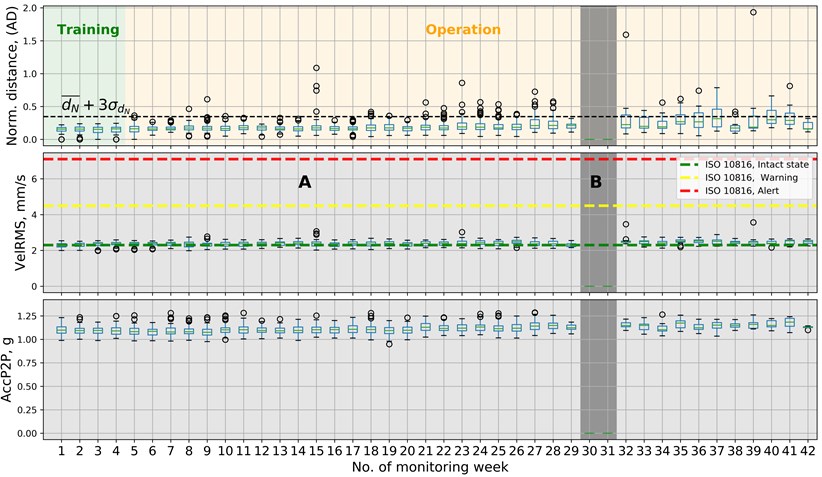
The anomaly detection analysis starts with establishing a normal region in multi-feature space, that represents the machine in its intact state. The first case study presented in Fig. 7 is performed on fan #1 just after the maintenance work. The DE bearing had to be replaced. Data for the training phase (in green) are selected from the first four weeks after the replacement of the bearing. Both training and operation phases are marked in Fig. 7. The normalized distance for weeks from no. 5 to no. 22 does not exceed the -threshold set for the AD algorithm. Only a few outliers between weeks 15 and 20 appeared to go beyond the threshold. The AD result changes at week no. 23 when the measurements start to move toward the established threshold. After the appearance of outliers in the week no. 23 a median also goes over the AD threshold in week 24. Then for the next 6 weeks, the results fluctuate on the edge of the threshold. From week no. 24 the median for every week till the end of the monitoring time stays over the AD threshold. Anomaly detection results are followed in Fig. 7 by the velocity RMS and acceleration peak to peak values also presented in the form of box plots. The time when the anomaly detection result changes from state OK (below the threshold) to NOK (above the threshold) is also followed by a change in the velocity RMS. Acceleration peak to peak stays for the whole monitoring time within the range of 0.8 to 1 g and does not change its state.
Fig. 7Anomaly detection, velocity RMS and acceleration peak-to-peak in a form of a box plots for CS I. A – intact state, B – fault condition C – machine turned off
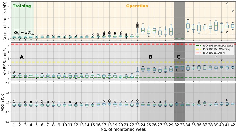
The monitoring period can be divided into three phases from the condition monitoring point of view. They are presented in Fig. 7 and listed in Table 2. From the AD perspective, monitoring time can be divided into two periods: training and testing.
Table 2Description of phases for case study I
Approach | Phase | Week no. |
Anomaly detection | Training | 1-4 |
Operation (testing) | 4-42 | |
Condition monitoring | Intact state of the machine (A) | 1-23 |
Fault condition detected at the fan (B) | 24-42 | |
Maintenance work on other machines, machine turned off (C) | 30-31 |
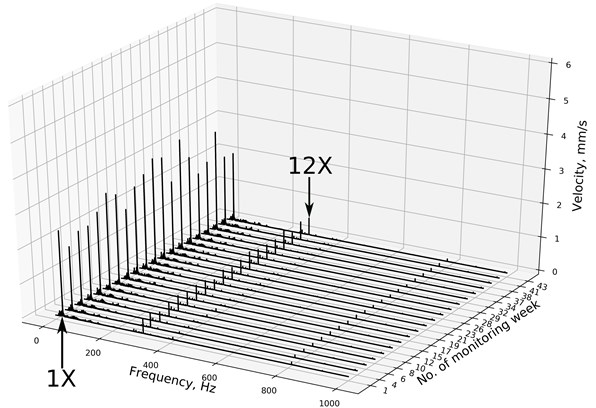
A raise in the velocity RMS may suggest many different types of fault conditions. Therefore, the frequency domain analysis of the signals is performed in Fig. 8 The velocity signal in the frequency domain is presented in a range between 0 and 1000 Hz. For each spectrum, the dominant frequency is 1X (rotational speed frequency). The second amplitude in every spectrum, which is also visible, is 12X (Blade Pass Frequency).
Fig. 8Waterfall diagram representing velocity spectra. 1X – rotational speed, 12X – Blade pass frequency for CSI, fan #1
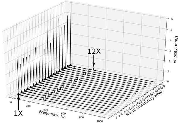
Change in the velocity RMS between week no. 23 and 24 corresponds with the raise of 1X amplitude. Other frequencies do not change their amplitudes significantly during the monitoring period. Distance increase detected by the AD algorithm (week no. 24) is caused by the raise of the rotational speed frequency amplitude. This kind of change in over-hung fans could be a reliable indicator of imbalanced growth, which in this case occurred due to uneven mass distribution at the rotor blades. Such fault condition is very common at monitored fans, and early information about growing imbalance helps to plan suitable maintenance works. In this case, AD performed similarly to the velocity RMS indicator what was the correct behavior of the algorithm. A fault was recognized as an anomaly in the same time as 1X (and velocity RMS) started to grow. Although AD in this form is not designed to interpret the data, it is a handy tool to raise an early alarm, which should be followed by an expert analysis of spectra and historical data. The maintenance crew confirmed the findings of both analyses. It is worth to mention that in this case thresholds set as default from the ISO standard (red and yellow dashed lines in Fig. 7) happens to be too high. There would be no diagnostic information from the system about the unbalance change without the anomaly detector. If maintenance procedure (in this case cleaning blades of the fan) are introduced early enough, it can prevent further deterioration of the machine and significantly extend its remaining useful life.
3.3. Case study II (Fan#2) deterioration of DE bearing
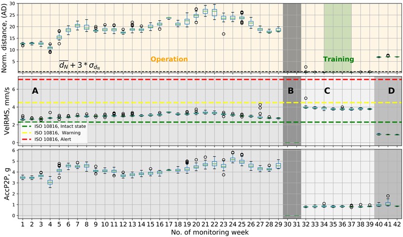
In the second case study, fan #2 was selected to perform the anomaly detection analysis. The first four weeks of monitoring time were chosen as a source of training data. In hindsight, the requirement that the machine was intact during the definition of a normal region was violated. It could be observed that the bearing fault was probably already present in the machine from the very beginning of its monitoring. The indications of the system are presented in Fig. 9. In the second week of its operation (past the end of the training period), the AD algorithm exceeded the threshold and returned anomaly indications until the end of the monitoring time.
The time-domain features collected within 42 weeks for fan #2 are presented below the AD results in Fig. 9. There are four phases of fan conditions marked in Fig. 9 with letters A, B, C, and D. From the beginning of the phase, the acceleration peak-to-peak indicator grew. This kind of trend can be the energy growth indicator in a high-frequency range, indicating some possible bearing problems. The velocity RMS also grew but not as fast as acceleration. Velocity RMS hits the apex at 21st week of monitoring. Acceleration peak to peak signal reaches the maximum value in the week no. 24. Afterward, all the indicators decreased slightly. Phase C starts with shutting down of the fan due to maintenance reasons. During the maintenance, the balancing procedure was performed at the rotor, and the DE bearing was replaced. A balanced rotor was installed in the machine again, and the velocity RMS went higher than before the maintenance procedure. To explain this unexpected behavior, the machine was turned off, and the balancing was performed again. Phase D represents measurements after the second balancing of the rotor. Features values in this phase are steady and low what was expected after the properly done maintenance work. All of the vibration parameters in phase D reach the minimal values within the data collection time. States of machine conditions for CSII and AD phases are listed in Table 3.
Fig. 9Anomaly detection, velocity RMS and acceleration peak-to-peak in a form of a box plots for CS II
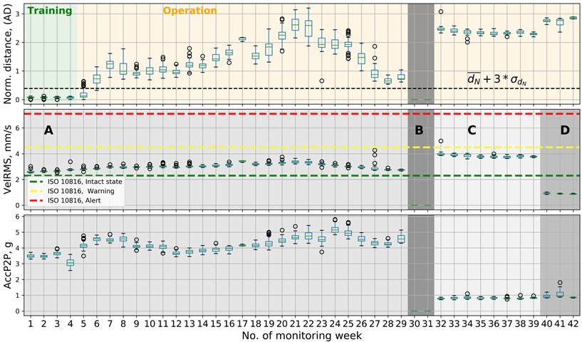
Table 3Description of phases for case study II
Approach | Phase | Week no. |
Anomaly detection | Training | 1-4 |
Operation | 5-42 | |
Condition monitoring | Development of bearing fault condition (A) | 1-29 |
Maintenance work: first balancing and bearing replacement (B) | 30-31 | |
Machine operation after the first maintenance (C) | 32-39 | |
Second balancing (corrected) and machine operation afterwards (D) | 40-42 |
It is worth to note that the intact state (phase D) of the machine is also recognized as an anomaly. This particular example proves that the anomaly detection approach shows the change but does not give information about whether the machine condition improved or decreased. For that reason, the anomaly indications appearing after the maintenance should be carefully investigated as they might mean that either the maintenance was not successful (as in between phases A and C) or that – while being successful – it resulted in a new normal state (as in between phases A and D). In the latter case, the system should be retrained prior to a further usage. Phase A and C are below the warning limit from ISO 10816-3 standard. Data after the second balancing procedure fall below the green line which means that maintenance procedures were done correctly.
An in-depth analysis of the phenomena occurring during case study II is performed based on velocity spectra. The spectra are presented in Fig. 10 in the form of a waterfall diagram.
Fig. 10Waterfall velocity spectra in monitoring period in case study II. BPFO is ball pass frequency of outer race. 2x and 4x are second and fourth harmonics of BPFO
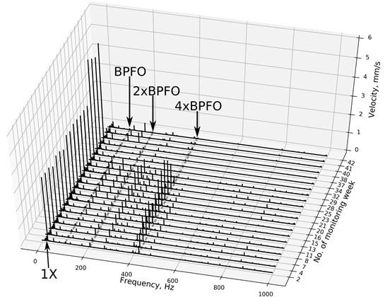
The growth of the velocity RMS in phase A is related to an increase in energy within the frequency range between 200 and 600 Hz. Dominating amplitudes in this frequency band grow from week no. 1 to 21 and fall down at week 22. These frequencies are harmonics of rotational speed frequency and fault frequencies, which can be associated with BPFO of DE (Drive End) bearing. Harmonics of 1X and the existence of BPFO indicate a problem with the bearing and possible looseness issue. The first order vibration (1X) amplitude within phase A stays steady. Frequencies in the range between 200 and 600 Hz decrease significantly in phases C and D. Due to the incorrect balancing procedure, the amplitude for rotational speed frequency increased in phase C. For this reason, the balancing procedure was performed once again and in the phase D all components characteristic for the fault condition decreased significantly in the spectrum.
3.4. Case study III (Fan #2) wrong balancing procedure (simulation approach)
Another approach to AD is based on data presented in CS II from the monitoring period of fan #2. AD was trained on data from the time when the machine was improperly balanced (weeks 32-39). It is rather the simulation approach because the operation phase is not only after the training phase but also before it. The results of this trial are presented in Fig. 11. The monitoring period is the same as in case study II, but the training phase is done in different weeks.
All measurements that were collected outside C phase are recognized anomalies. Furthermore, data from D phase (intact state of the machine) are also recognized anomalies. This case study shows that the data interpretation must follow anomaly detection applications. It gives information about the change that occurred in the system but does not necessarily mean that it had to be a fault condition.
Fig. 11CS III at fan #2, AD trained in weeks no. 34-37
3.5. Case study IV (Fan #3) intact state monitoring
In the last case study, data gathered on fan #3 are presented in Fig. 12.
Fig. 12AD, velocity RMS and acceleration peak-to-peak results for CS IV, no fault at the fan #3
Since no problems with the operation of the machine were detected, only two phases are marked in figures. Phase A is the operation phase, and phase B represents the time when fan #3 was turned off due to maintenance works done on the other fans. There are weeks when single anomalies are detected, but a median indication for a week did not cross the AD threshold. There is no clear change of the state in case of fan #3. Since the state of the machine was known to be intact, all of AD indications can be treated as false positives. Therefore, the method exhibits a 3 % false-positive rate measurement-wise and 0 % false-positive rate week-wise.
Fig. 13 presents velocity spectra according to weeks of the monitoring. There are two significant frequencies in Fig. 13, and both are described with an arrow (1X and 12X). The rotational speed frequency oscillates within the monitoring period, but it cannot be associated with a new state of machine condition as easily as in CSI-III. Those changes are rather effects of different operational conditions within the monitoring time. They might be caused by such factors like temperature, transient changes at the machine, or industrial process. These findings are consistent with the feedback from the maintenance crew – state of Fan #3 was deemed OK for the whole monitoring period and well after the end of it. Up to the date of this paper submission, no faults were detected in Fan #3.
Fig. 13Waterfall diagram for fan #3, CS IV. 1X – rotational speed frequency, 12X – blade pass frequency
4. Summary and conclusions
4.1. Results discussion
The new anomaly detection algorithm for rotating machinery was proposed in the hereby article. The algorithm, inspired by optimal baseline selection techniques and the nearest-neighbor principle, was validated in four industrial case-studies. Four signal features were used as inputs to the algorithm. The learning dataset consisted of 2880 measurement points. The reduction of the training dataset to MRD containing 50 data samples, reduced the number of computations for every point in the testing (operational) dataset by 57.6 times. Data for growing imbalance, maintenance changes, intact state, and slowly increasing deterioration of a bearing were analyzed. The MRD-NN algorithm correctly labeled all of the cases. Classical time and frequency domain analyses proved to be appropriate for the interpretation of states recognized as anomalies. Once the anomaly detection method was trained on the intact state of the machine, the normalized distance to the normal region reflected the severity of the faults. The threshold from the AD algorithm was - in all cases - more sensitive to the change at the machine than thresholds applied from ISO standards. The proposed method proved to be operational and allowed for an efficient data reduction. The selection of a threshold using a rule employed for MRD was correct, as the number of false positives after week-wise data aggregation was 0 %, while still allowing for an efficient damage detection. The presented AD does not give interpretation to all possible fault conditions which might occur at the machine. On the other hand, it is a handy tool to inform about the change of the machine state. A strong advantage of this algorithm constitutes a fact that the feedback given from a combination of features is more robust, in terms of detection of faults, than the analysis of each feature individually.
4.2. Future work
This research has potential limitations. These limitations together with aspects, which can be developed in more detail in the future work on the subject are listed below:
– Monitoring period presented in the paper could be longer for this kind of machines to see the long-term trend of a deterioration in data.
– Performance of the algorithm on other kinds of defects e.g. related to the electric motor is one of interesting options for the next research steps.
– Further research in the field of a larger number of features included in the anomaly detector. Those can be related not only to vibrations but also to performance indicators such as: load, flow, temperature, etc. That would be especially valuable for IIoT applications.
– There is a lot of potential in looking for information that can be transferred within the same type of machines. Thus, the population based approach would be for sure also a very strong point to consider in the future research of the subject.
4.3. Conclusions
The most important findings of the work are as follows:
– The AD algorithm can be also used in cases when the initial machine state is already damaged, provided that the damage severity grows over time. This feature does not apply for cases when the machine state is not correct from the maintenance point of view but does not contain any structural damage - as seen in Case study III.
– The reduction of source data to MRD does not reduce the efficiency of the algorithm. It also provides an intuitive way of the threshold selection.
– The algorithm does not generate excessive false positive indications which allows its usage in practical industrial scenarios.
– The usage of MRD in the case of a four-week training dataset decreases the number of computations 57 fold.
– Thresholds from AD algorithm based on rule were more sensitive to changes in the machine condition than limits from ISO standard.
References
-
Dinardo G., Fabbiano L., Vacca G. A smart and intuitive machine condition monitoring in the Industry 4.0 scenario. Measurement: Journal of the International Measurement Confederation, Vol. 126, 2018, p. 1-12.
-
Hamrol A., Gawlik J., Sładek J. Mechanical engineering in industry 4.0. Management and Production Engineering Review, Vol. 10, Issue 3, 2019, p. 14-28.
-
Sanghavi D., Parikh S., Aravind Raj S. Industry 4.0: Tools and implementation. Management and Production Engineering Review, Vol. 10, Issue 3, 2019, p. 3-13.
-
Ju H., Wang X., Zhang T., Zhao Y., Ullah Z. Defect recognition of buried pipeline based on approximate entropy and variational mode decomposition. Metrology and Measurement Systems, Vol. 26, Issue 4, 2019, p. 739-755.
-
Urbanek J., Barszcz T., Uhl T. Comparison of advanced signal-processing methods for roller bearing faults detection. Metrology and Measurement Systems, Vol. 19, Issue 4, 2012, p. 715-726.
-
Girdhar P., Scheffer C. Practical Machinery Vibration Analysis and Predictive Maintenance. Elsvier, 2004.
-
Dworakowski Z., Ambroziński L., Stępiński T. Multi-stage temperature compensation method for Lamb wave measurements. Journal of Sound and Vibration, Vol. 382, Issue 25, 2016, p. 328-339.
-
Dworakowski Z., Dziedziech K., Jabłoński A. A novelty detection approach to monitoring of epicyclic gearbox health. Metrology and Measurement Systems, Vol. 25, Issue 3, 2016, p. 328-339.
-
Lis A., Dworakowski Z., Czubak P. Anomaly detection approach for fan monitoring, an industrial case study. 9th European Workshop on Structural Health Monitoring, Manchester, United Kingdom, 2018.
-
Randall R. B. Vibration-Based Condition Monitoring: Industrial, Aerospace and Automotive Applications. Wiley, 2010.
-
Cha Y.-J., Wang Z. Unsupervised novelty detection based structural damage localization using a density peaks-based fast clustering algorithm. Structural Health Monitoring, Vol. 17, 2007, p. 13-324.
-
Schmit S., Heyns P.S., de Villiers J. P. A novelty detection diagnostic methodology for gearboxes operating under fluctuating operating condition using probabilistic techniques. Mechanical Systems and Signal Processing, Vol. 100, 2018, p. 152-166.
-
Dervills N., Choi M., Taylor S., Barthorpe R. B., Park G., Farrar C., Worden K. On damage diagnosis for a wind turbine blade using pattern recognition. Journal of Sound and Vibration, Vol. 333, 2014, p. 1833-1850.
-
Cury A., Cremona C., Dumoulin J. Long-term monitoring of a PSC box grider bridge: Operational modal analysis, data normalization and structural modification assessment. Mechanical Systems and Signal Processing, Vol. 99, 2014, p. 215-249.
-
Pimentel M. A., Clifton D. A., Clifton L., Tarassenko L. A review of novelty detection. Signal Processing, Vol. 99, 2014, p. 215-249.
-
Markou M., Singh S. Novelty detection: a review – part 1: neural network based approaches. Signal Processing, Vol. 83, 2003, p. 2481-2497.
-
Markou M., Singh S. Novelty detection: a review – part 2: neural network based approaches. Signal Processing, Vol. 83, 2003, p. 2499-2521.
-
Worden K., Manson G., Fieller N. Damage detection using outlier analysis. Journal of Sound and Vibration, Vol. 229, 2000, p. 647-667.
-
Surace C., Worden K. Novelty detection in a changing environment: A negative selection approach. Mechanical Systems and Signal Processing, Vol. 24, 2010, p. 1114-1128.
-
Dhami S. S., Pabla B. S. Hybrid data fusion approach for fault diagnosis of fixed-axis gearbox. Structural Health Monitoring, Vol. 17, Issue 4, 2017, p. 936-945.
-
Zhang S., Zhang Y., Li L., Wang S., Xiao Y. An effective health indicator for rolling elements bearing based on data space occupancy. Structural Health Monitoring, Vol. 17, 2016, p. 3-14.
-
Jin S.-S., Jung H.-J. Vibration-based damage detection using online learning algorithm for output-only structural health monitoring. Structural Health Monitoring, Vol. 17, 2017, p. 727-746.
-
Urbanek J., Barszcz T., Sawalhi N., Randall R. B. Comparison of amplitude-based and phase-based methods for speed tracking in application to wind turbines. Metrology and Measurement Systems, Vol. 8, Issue 2, 2011, p. 295-304.
-
Zimroz R., Urbanek J., Barszcz T., Bartelmus W., Millios F., Martin N. Measurement of instantaneous shaft speed by advanced vibration signal processing – application to wind turbine gearbox. Metrology and Measurement Systems, Vol. 18, Issue 4, 2011, p. 701-712.
-
Lei Y. Intelligent Fault Diagnosis and Remaining Useful Life Prediction of Rotating Machinery. Elsvier, 2016.
-
Chudzikiewicz A., Bogacz R., Kostrzewski M. Using acceleration signals recorded on a railway vehicle wheelsets for rail track condition monitoring. 7th European Workshop on Structural Health Monitoring, Nantes, 2014, p. 167-174.
-
Feng G., Zhao H., Gu F., Needham P., BallA. D. Efficient implementation of envelope analysis on resources limited wireless sensor nodes for accurate bearing fault diagnosis. Measurement: Journal of the International Measurement Confederation, Vol. 110, 2017, p. 307-318.
-
Elasha F., Greaves M., Mba D. Planetary bearing defect detection in a commercial helicopter main gearbox with vibration and acoustic emission. Structural Health Monitoring, Vol. 17, Issue 5, 2018, p. 1192-1212.
-
Kim J.-S., Lee S.-K. Identification of tooth fault in a gearbox based on cyclostationarity and empirical mode decomposition. Structural Health Monitoring, Vol. 17, Issue 3, 2017, p. 494-513.
-
Muralidharan V., Sugumaran V. Feature extraction using wavelets and classification through decision tree algorithm for fault diagnosis of mono-block centrifugal pump. Measurement: Journal of the International Measurement Confederation, Vol. 46, Issue 1, 2013, p. 353-359.
-
Elforjani M. Diagnosis and prognosis of slow speed bearing behavior under grease starvation condition. Structural Health Monitoring, Vol. 17, Issue 3, 2018, p. 532-548.
-
Fei C.-W., Choy Y.-S., Bai G.-C., Tang W.-Z. Multi-feature entropy distance approach with vibration and acoustic emission signals for process feature recognition of rolling element bearing faults. Structural Health Monitoring, Vol. 17, Issue 2, 2018, p. 156-168.
-
Osowski S., Siwek K. Mining data of noisy signal patterns in recognition of gasoline bio-based additives using electronic nose. Metrology and Measurement Systems, Vol. 24, Issue 1, 2017, p. 27-44.
-
Worden K., Cross E., Dervilis N., Evangelos P., Ifigenia A. Structural health monitoring: from structures to systems-of-systems. IFAC-PapersOnLine, Vol. 48, Issue 21, 2015, p. 1-17.
-
AC102 Datasheet, https://documents.ctconline.com/datasheet?type=Sensor&prd=AC102.
Cited by
About this article

The work presented in this article was supported by the National Centre for Research and Development in Poland under project No. POIR.01.02.00-0016. This research was made possible due to data provided by R&D Department of the Elmodis Company.
