Periodic non-sinusoidal time-delay stochastic resonance weak fault diagnosis method and its application

1. Introduction

Fault detection technology in industrial production for mechanical equipment has received recent attention. This is because equipment failure can cause equipment damage and also affect personnel safety [1, 2]. Because large mechanical equipment is often operated at low-speed in heavy-duty and noisy working environments, it can be difficult to identify early warnings of failure [3]. Early fault signals in key parts (e.g., bearings) are often difficult to detect in noisy settings and can lead to inaccurate fault diagnosis [4]. Therefore, for early fault detection, the ability to extract weak fault characteristics within a noisy background is important [5].

A variety of signal processing methods have been proposed and studied. These include empirical mode decomposition [6, 7], wavelet analysis [8, 9], and singular value decomposition [10, 11]. These methods are primarily based on noise reduction, having the potential to weaken the weak fault characteristic signal while processing noise [12]. Some scholars have developed fault detection systems based on traditional signal processing algorithms. These include supervised learning systems that predict performance and remaining life of bearings and other components [13-15]. Stochastic resonance (SR), on the other hand, uses a different approach for filtering noise. It adds moderate noise that can excite the particles in the nonlinear system and enhance the amplitude and power of the weak signal.

SR was first proposed by Benzi [16] as a method to detect weak faults in paleo-meteorological glaciers. Since then, SR has been applied to meteorology, biology, and physics [17-21]. Recently, SR has been used for mechanical fault detection [22, 23]. Early fault detection SR studies aimed to overcome small parameter limits (e.g., fault frequency < 1 Hz) [24-26]; however, the actual fault frequency is typically greater than 1 Hz. Lu et al. [27] developed an embedded system based on multi-scale noise-tuned SR and applied it to train signal detection. Lei et al. [28] proposed an adaptive signal processing mechanism and applied it to fault detection of missing or broken teeth. Qiao et al. [12] researched an unsaturated SR to overcome the output saturation problem of classic bi-stable SR (CBSR). This application effectively improved the signal-to-noise ratio (SNR). Lei et al. [29] investigated under-damped SR on the synergistic effect of the damping factor and vibration signal. It was shown to obtain both a higher amplitude and larger SNR output. Shi et al. [30] proposed multiple fault frequency detection to the background of color noise. Lu et al. [31] investigated an SR mechanism for the Woods-Saxon potential function. This could detect weak signals at different noise levels. Lu et al. [32] proposed a tri-stable SR model that could further amplify the SNR in low SNR signal detection settings.

All of the aforementioned SR studies are considered to be short-term memory systems as they do not consider historical information. A time-delay feedback SR uses historical information of the original system and applies it to the negative feedback to form a new system. This may improve the detection of weak periodic signals; however, few studies have been conducted using this method. Two examples are Lu et al. [33] and Shi et al. [34]. Lu et al. [33] used a time-delay CBSR weak fault detection method for the purpose of analyzing bearings; Shi et al. [34] investigated the SR of a three-stable system with a time-delay feedback. Although these two methods considered time-delay, both were directed to bi-stable or tri-stable nonlinear systems with a single potential structure. Therefore, it is impossible to form a perfect nonlinear system structure and match complex vibration signals. The synergy between time-delay feedback, system parameters, and vibration signals is also not considered which can affect the enhancement ability of SR. Furthermore, the global optimization ability of genetic algorithms, time-delay feedback, system parameters, and vibration signals is synergistic. Therefore, these should also be included to achieve the best SNR output using the most optimal parameter settings.

This paper presents a periodic non-sinusoidal time-delay SR (PNTSR) model and applies it to bearing fault detection. The PNTSR model has a richer potential model structure with coefficients that can be adjusted to better match with the complex vibration signals. The time-delay is introduced on the basis of a traditional SR system, allowing the model to incorporate the influence of historical factors. The second part of this paper analyzes the characteristics of the PNTSR model and discusses the effective potential function (EPF), steady-state probability density function (SPDF), and SNR. The third part describes the weak fault detection strategy and simulation for the PNTSR model. The paper then verifies the PNTSR method using experimental and engineering data and concludes with a summary of the findings.

2. PNTSR introduction

2.1. Model of PNTSR

SR is the synergy between noise and weak signals in a nonlinear system. The appropriate amount of noise and weak signals are used to drive the particles to move periodically into the potential wells on both sides to detect weak signals. CBSR methods are based on the bi-stable potential model:

1

$U_c\left(x\right)=\frac{1}{2}a{x}^2+\frac{1}{4}b{x}^4,$

where $a$ and $b$ are non-zero values. By adjusting $a$ and $b$, different potential model shapes can be obtained. However, this article introduces a new potential model [35]:

2

$U\left(x\right)=U_0{\left(1-r\right)}^2\frac{1-\mathrm{c}\mathrm{o}\mathrm{s}x}{\left(1+r^2+2r\mathrm{c}\mathrm{o}\mathrm{s}x\right)}.$

Fig. 1The shape of Ux depends on the parameterr. Assuming U0=1, Ux is plotted for a) r= –0.6, b) r= 0, c) r= 0.4, and d) r= 0.6

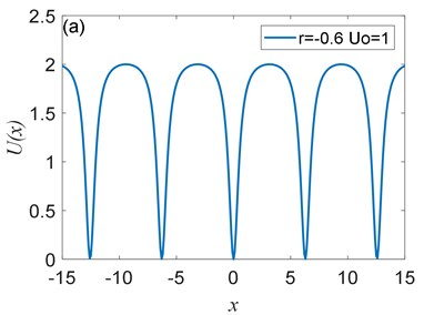
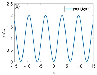
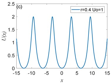
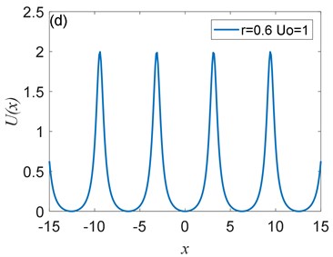
Fig. 2The peak value of Ux depends on U0: a) U0= 0.1, b) U0= 0.25, c) U0= 0.5, d) U0= 0.75, where r= 0.4

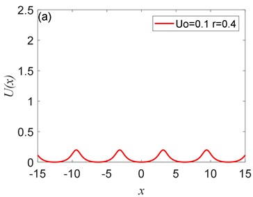
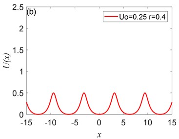
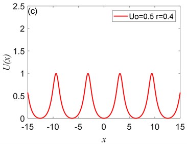
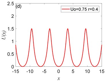
The potential has periodicity but belongs to a non-sinusoidal function, and the period is 2$\pi$ (Fig. 1, Fig. 2). As you can see from Fig. 1 that the parameter $r$ determines the roundness of the barrier and the width of the potential well. The smaller parameter $r$ is, the smoother the barrier will be, and the potential well becomes wider. Fig. 2 illustrates that the parameter $U_0$ controls the peak of the barrier, the larger $U_0$, the higher the barrier. Therefore, adjusting the size of the parameters $r$ and $U_0$ determines the shape of the potential structure. Comparing with the CBSR system, the periodic non-sinusoidal potential model has multiple potential wells, when the noise is too large, multiple potential wells can absorb part of the noise energy and reduce noise interference; the periodic non-sinusoidal potential model can achieve independent adjustment of the well width and the barrier height, and a richer potential model structure can be formed by adjusting the parameters.

2.2. Impact of the time-delay feedback on EPF, SPDF, and SNR

Time-delay feedback SR is based on CBSR, which introduces historical information from the original short-term memory system to the long-term memory system, and the classical bi-stable delay system is:

3

$\frac{dx\left(t\right)}{dt}=x\left(t\right)-x^3\left(t\right)+\lambda x\left(t-\tau \right)+A\mathrm{c}\mathrm{o}\mathrm{s}\left(\mathrm{\Omega }t\right)+\sqrt{2D}\xi \left(t\right).$

$A\mathrm{c}\mathrm{o}\mathrm{s}\left(\mathrm{\Omega }t\right)$is a extracted signal, $A$ is signal strength, and $\mathrm{\Omega }$ represents the phase. $\lambda$ represents the feedback strength, $\tau$ represents the time-delay. $D$ stands for noise intensity, $\xi \left(t\right)$ stands for external noise. We consider a delay period non-sinusoidal potential system driven by a weak periodic signal. Substituting Eq. (2) into Eq. (3) gives:

4

$\frac{dx\left(t\right)}{dt}=U_0{\left(1-r\right)}^2\frac{\mathrm{s}\mathrm{i}\mathrm{n}x\left(t\right)+2r\mathrm{s}\mathrm{i}\mathrm{n}x\left(t\right)\left(1-\mathrm{c}\mathrm{o}\mathrm{s}x\left(t\right)\right)}{{\left(1+r^2+2r\mathrm{c}\mathrm{o}\mathrm{s}x\left(t\right)\right)}^2}$
$+\lambda x\left(t-\tau \right)+A\mathrm{c}\mathrm{o}\mathrm{s}\left(\mathrm{\Omega }t\right)+\sqrt{2D}\xi \left(t\right).$

Eq. (4) is a non-Markov that needs to be simplified to a Markov process. The Fucker Plane is as follows [36]:

5

$\frac{\partial p\left(x,t\right)}{\partial t}=\frac{\partial \left[h_{eff}p\left(x,t\right)\right]}{\partial x}+D\frac{{\partial }^{2}p\left(x,t\right)}{\partial x^2},$

where $h_{eff}$ represents the conditional average drift rate to satisfy:

6

$h_{eff}={\int }_b^{a}d{x}_{\tau }h\left(x,x_{\tau }\right)p\left(x_{\tau },t-\tau |x,t\right),$

where:

7

$x_{\tau }=x\left(t-\tau \right),$

8

$h\left(x,x_{\tau }\right)=U_0{\left(1-r\right)}^2\frac{\mathrm{s}\mathrm{i}\mathrm{n}x\left(t\right)+2r\mathrm{s}\mathrm{i}\mathrm{n}x\left(t\right)\left(1-\mathrm{c}\mathrm{o}\mathrm{s}x\left(t\right)\right)}{{\left(1+r^2+2r\mathrm{c}\mathrm{o}\mathrm{s}x\left(t\right)\right)}^2}+\lambda x_{\tau }+A\mathrm{c}\mathrm{o}\mathrm{s}\left(\mathrm{\Omega }t\right),$

9

$h\left(x\right)=U_0{\left(1-r\right)}^2\frac{\mathrm{s}\mathrm{i}\mathrm{n}x\left(t\right)+2r\mathrm{s}\mathrm{i}\mathrm{n}x\left(t\right)\left(1-\mathrm{c}\mathrm{o}\mathrm{s}x\left(t\right)\right)}{{\left(1+r^2+2r\mathrm{c}\mathrm{o}\mathrm{s}x\left(t\right)\right)}^2}+\lambda x+A\mathrm{c}\mathrm{o}\mathrm{s}\left(\mathrm{\Omega }t\right).$

$p\left(x_{\tau },t-\tau |x,t\right)$ is the zero-order approximate Markov transition probability density [37]:

10

$p\left(x_{\tau },t-\tau |x,t\right)=\frac{1}{\sqrt{4\pi D\tau }}\mathrm{e}\mathrm{x}\mathrm{p}\left(-\frac{\left(x_{\tau }-x-h\left(x\right){\tau }^2\right)}{4D\tau }\right).$

Eq. (10) brings in Eq. (6) and we get:

11

$h_{eff}=\left(1+\lambda \tau \right)U_0{\left(1-r\right)}^2\frac{\mathrm{s}\mathrm{i}\mathrm{n}x\left(t\right)+2r\mathrm{s}\mathrm{i}\mathrm{n}x\left(t\right)\left(1-\mathrm{c}\mathrm{o}\mathrm{s}x\left(t\right)\right)}{{\left(1+r^2+2r\mathrm{c}\mathrm{o}\mathrm{s}x\left(t\right)\right)}^2}$
$+\lambda \left(1+\lambda \tau \right)+\left(1+\lambda \tau \right)A\mathrm{c}\mathrm{o}\mathrm{s}\left(\mathrm{\Omega }t\right).$

Further derivation can get an Equivalent Langevin equation:

12

$\begin{array}{l}\frac{dx\left(t\right)}{dt}=U_0{\left(1-r\right)}^2\frac{\mathrm{s}\mathrm{i}\mathrm{n}x\left(t\right)+2r\mathrm{s}\mathrm{i}\mathrm{n}x\left(t\right)\left(1-\mathrm{c}\mathrm{o}\mathrm{s}x\left(t\right)\right)}{{\left(1+r^2+2r\mathrm{c}\mathrm{o}\mathrm{s}x\left(t\right)\right)}^2}+\lambda x+A\mathrm{c}\mathrm{o}\mathrm{s}\left(\mathrm{\Omega }t\right)\\ +\lambda \tau \left[U_0{\left(1-r\right)}^2\frac{\mathrm{s}\mathrm{i}\mathrm{n}x\left(t\right)+2r\mathrm{s}\mathrm{i}\mathrm{n}x\left(t\right)\left(1-\mathrm{c}\mathrm{o}\mathrm{s}x\left(t\right)\right)}{{\left(1+r^2+2r\mathrm{c}\mathrm{o}\mathrm{s}x\left(t\right)\right)}^2}+\lambda x+A\mathrm{c}\mathrm{o}\mathrm{s}\left(\mathrm{\Omega }t\right)\right]+\sqrt{2D}\xi \left(t\right).\end{array}$

Without considering the periodic signal, the EPF can be derived as:

13

$U_{eff}\left(x\right)=\left(1+\lambda \tau \right)\left(U_0\left(1-r\right)\frac{1-\mathrm{c}\mathrm{o}\mathrm{s}x}{1+r^2+2r\mathrm{c}\mathrm{o}\mathrm{s}x}\right)+\frac{1}{2}\lambda \left(1+\lambda \tau \right)x^2.$

The effect of different $\lambda$ and $\tau$ on the EPF is shown in Fig. 3.

Fig. 3Different λ and τ for EPF

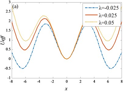
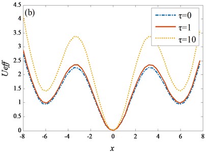
Fig. 3(a) shows that as $\lambda$ increases, the potential wells on both sides of the zero point become lower, the barrier is relatively lower, and the round trip of the particles between the potential wells becomes easier. In Fig. 3(b), with the increase of $\tau$, the potential wells on both sides of the zero point rise, and it is easier for the particles to transition from one side well to the other. Comparing Fig. 3(a) and 3(b), it can be noted that the $\lambda$ is more sensitive to the adjustment EPF than the $\tau$. The time delay $\tau$ varies from 1 to 10, and the EPF changes significantly, while the feedback strength requires only a small parameter variation range. With further calculation, we obtain the SPDF expression:

14

$p_{st}=N\mathrm{e}\mathrm{x}\mathrm{p}\left(-\frac{U_{eff}}{D}\right),$

where $N$ is the normalized constant. The SPDF is shown in Fig. 4.

Fig. 4Different λ and τ for SPDF

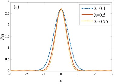
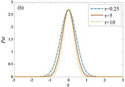
Different values of $\lambda$ have no effect on the peak of the SPDF (Fig. 4(a)). As $\lambda$ increases, the SPDF is more concentrated. Figs. 4(b) and 4(a) have similar properties. As $\tau$ increases, the peak of SPDF does not change. Comparing the two figures, the effect of the feedback strength $\lambda$ is more sensitive than the effect of the time-delay time $\tau$ on the SPDF. Subsequently the power spectral density can be derived as [38]:

15

$S\left(\omega \right)=S_1\left(\omega \right)+S_2\left(\omega \right)=\frac{\pi \left(1+\lambda \right)M^2}{2\left(N^2+{\mathrm{\Omega }}^2\right)}\left[\delta \left(\mathrm{\Omega }-\omega \right)+\delta \left(\mathrm{\Omega }+\omega \right)\right]$
$+\left[1-\frac{M^2}{2\left(N^2+{\mathrm{\Omega }}^2\right)}\right]\frac{2\left(1+\lambda \right)N}{N^2+{\omega }^2},$

where $S_1\left(\omega \right)$ and $S_2\left(\omega \right)$ is the power spectrum of the useful signal and external noise, respectively. $N$ and $M$ are as follows:

16

$N=\frac{\sqrt{2}\left(1+\lambda \right)\left(1+\lambda \tau \right)}{\pi }\mathrm{e}\mathrm{x}\mathrm{p}\left(-\frac{{\left(1+\lambda \right)}^2\left(1+\lambda \tau \right)}{4D}\right),$

17

$M=\frac{A}{D}\left(1+\lambda \tau \right)\sqrt{1+\lambda }N.$

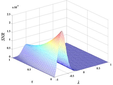
Subsequently, the output SNR can be expressed as $S_1\left(\omega \right)/S_2\left(\omega \right)$. Substituting $S_1\left(\omega \right)$ and $S_2\left(\omega \right)$ gives:

18

$SNR=\frac{S_1\left(\omega \right)}{S_2\left(\omega \right)}=\frac{\sqrt{2}{A}^2}{4D^2}{\left(1+\lambda \right)}^2{\left(1+\lambda \tau \right)}^3\mathrm{e}\mathrm{x}\mathrm{p}\left[-\frac{{\left(1+\lambda \right)}^2\left(1+\lambda \tau \right)}{4D}\right].$

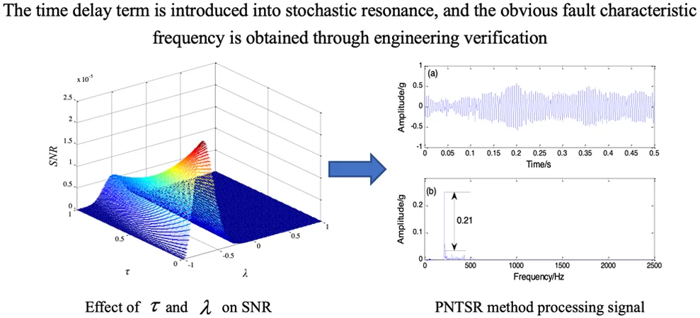
As shown in Fig. 5, as the feedback strength $\lambda$ increases, the SNR tends to increase first and then decrease. Since noise intensity at the detection of a weak fault signal is fixed, the optimum SNR should be obtained by changing the delay term.

3. Detection strategy and simulation for the PNTSR

3.1. Detection strategy for the PNTSR method

Because the realization condition of SR is under the adiabatic approximation theory, it satisfies the small parameter requirement. Therefore, the frequency shift variable scale to change signal scale, and then use the fourth-order Runge-Kutta method and get the output. SNR is the evaluation index. The definition of SNR is:

19

$SNR=10\mathrm{l}\mathrm{o}{\mathrm{g}}_{10}\frac{A_d^2}{{\sum }_{i=1}^{N/2}{A}_i^2-A_d^2},$

where $N$ represent the data length, and $A_d^2$ and ${\sum }_{i=1}^{N/2}{A}_i^2-A_d^2$ correspond to the amplitude of the extracted signal and the external noise. The genetic algorithm is used to adjust the parameters $U_0$, $r$, $\lambda$ and $\tau$ to match the complex vibration signals to obtain the optimal output. Therefore, we get the PNTSR fault detection method flow:

(1) Data preprocessing. The signal demodulation methods such as band pass filtering and envelope extraction are used to obtain the driving signal. The small parameter limitation is solved by the frequency shift variable scale.

(2) Parameter initialization. Initialize the potential system parameters, time extension and feedback strength, and use SNR as the output evaluation index.

(3) Parameter optimization. Using the global optimization ability of the genetic algorithm, the system parameters, time-delay feedback and complex vibration signals work together to obtain the optimal values of system parameters, time-delay, and feedback strength.

(4) Output calculation. The result output is calculated by Eq. (14), and then the SNR is calculated by Eq. (15) to ensure the best combination of parameters.

(5) Signal post processing. The optimal parameters are substituted into the potential model to obtain the optimal filtering, which is the spectrum, to realize the identification and diagnosis of fault characteristics.

Fig. 5Effect of time-delay τ and feedback strength λ on SNR

The specific flow chart is as follows (Fig. 6).

3.2. Simulation verification of PNTSR method

To verify the PNTSR method, the PNTSR method is analyzed by simulating the rolling bearing fault signal. The simulation signal is generated by the following formula:

20

$S\left(t\right)=\mathrm{e}\mathrm{x}\mathrm{p}\left\{-d{\left[t-n\left(t\right)T_d\right]}^2\right\}\cdot A\mathrm{s}\mathrm{i}\mathrm{n}\left(2\pi ft\right),$

where $A$ represents the signal strength, $d$ represents the reaction signal attenuation, $n\left(t\right)$ which control pulse period. $f=$ 79 Hz is the fault frequency. Moreover, the PNTSR method is contrast CBSR to emphasize that PNTSR is more effective.

The simulated clean signal and the noisy signal are shown in Fig. 7(a) and Fig. 7(b), respectively, and the corresponding spectrogram is seen in Fig. 7(c). Fig. 7(d) shows the resulting envelope spectrum. The spectrum and envelope extraction reveal that the useful signal is completely hidden, and fault signal cannot be detected.

Fig. 6Weak signal detection strategy for PNTSR

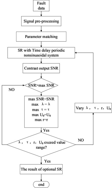
Fig. 7Bearing simulation data: a) clean data; b) noisy signal; c) spectrogram; d) envelope spectrogram

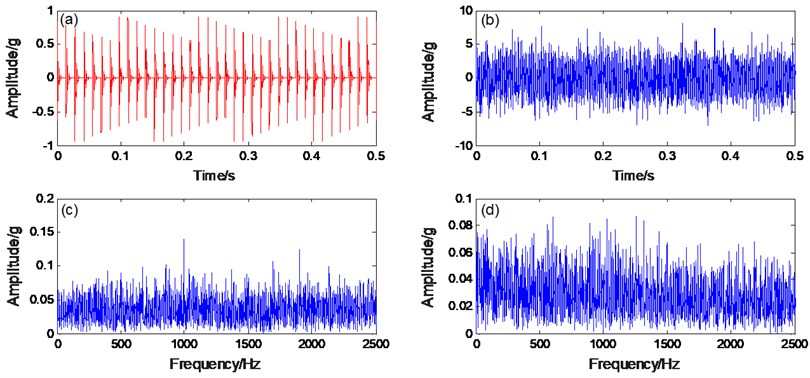
Fig. 8a) PNTSR processing signal, b) spectrogram, c) CBSR processing signal, d) spectrogram

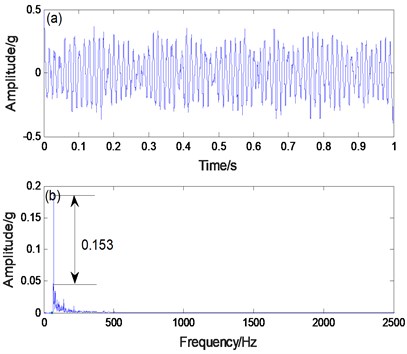
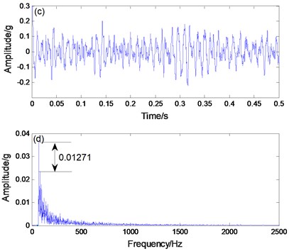
In order to extract the simulated rolling bearing fault signal, the simulated fault signal is applied to the CBSR and the PNTSR. Here, the distance between the amplitude of surrounding noise and the amplitude of simulated data is represented by the recognition degree. Comparing Figs. 8(b) and 8(d), the recognition degree of PNTSR method is 0.153, and the recognition degree of CBSR method is 0.01271. In Fig. 8(b), it is apparent that the primary frequency is the fault characteristic frequency and the other noises are smaller. In Fig. 8(d), the signal is more seriously affected by noise. Thus, we can conclude that the PNTSR has better extraction results.

4. Experimental verification of PNTSR method

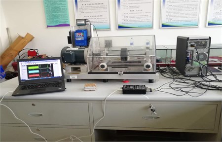
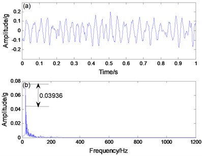
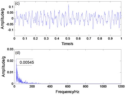
In the next step, we use the proposed method to detect bearing inner ring with slight wear faults in the laboratory. The experimental platform is a comprehensive bench for mechanical equipment (Fig. 9). The rotational frequency is 40 Hz, the experimental sampling frequency is 5120 Hz, and the bearing inner ring frequency is 217.28 Hz. The processed bearing fault signal is displayed in Fig. 10. In Fig. 10(b), the fault frequency is difficult to recognize due to interference from multiple high frequency and low frequency noise. However, in Fig. 10(c), although the useful signal frequency of 216 Hz, and seriously interfered by low frequency noise.

Fig. 9Bearing fault simulation platform

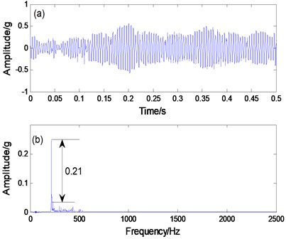
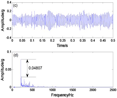
We apply the proposed method to the extraction fault feature of the bearing. Fig. 11(b) shows the spectrum output result. The fault frequency is the dominant frequency and the noise component is less affected. The recognition degree of the PNTSR method is 0.21. In Fig. 11(d), the CBSR output shows that the recognition degree of the faulty constant frequency is 0.04807. Therefore, we can conclude that the PNTSR is further better effective than CBSR in the bearing signal diagnosis.

Fig. 10a) Bearing signal, b) spectrogram, c) envelope spectrogram

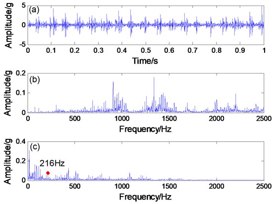
Fig. 11a) PNTSR processing signal, b) spectrogram, c) CBSR processing signal, d) spectrogram

5. Engineering verification of PNTSR method

In view of the good results, we apply the proposed method to engineering practice. The experimental object used is the rolling bearing of a steel mill and its inner ring fault characteristics are identified (Fig. 12). The bearing inner ring useful signal frequency is 24 Hz. The processed data is shown in Fig. 13. Because noise is large, the signal contour in the time domain graph is very inconspicuous. In Fig. 13(b), the extracted signal frequency of 24.3 Hz is hidden in the noise and cannot be discerned. Therefore, applying the PNTSR method processing signal can be seen in Fig. 14(a) and (b), which indicates that the signal profile in the time domain graph is relatively clear. In Fig. 14(b), the extracted signal frequency of 24.32 HZ, other noise interference is small, and the recognition degree of PNTSR method is 0.325. The collected data are applied to the CBSR method, the processed signal can be obtained, as shown in Figs. 14(c) and (d). The CBSR method has a large noise interference and the recognition degree is only 0.023 (Fig. 14d). Therefore, we can conclude that the proposed method not only has good signal extraction effects in simulation and experiments, but is also effective in practical engineering.

Fig. 12Fault detection of the bearing inner ring of the steel mill.

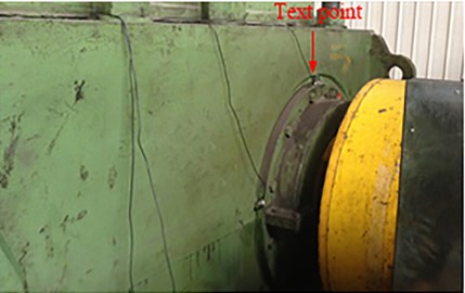
Fig. 13a) Engineering verification bearing signal, b) spectrogram, c) envelope spectrogram

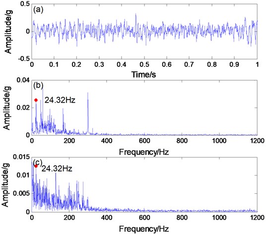
Fig. 14a) PNTSR processing signal, b) spectrogram, c) CBSR processing signa, d) spectrogram

6. Conclusions

In this paper, the PNTSR system was investigated and a method for diagnosing weak faults was proposed. Following are the conclusions from this paper:

1) The introduced periodic non-sinusoidal potential function consists of two structural parameters $U_0$ and $r$. These can be adjusted to obtain a variety of potential models. Notably, transitions are more abundant.

2) The PNTSR system is a multiple potential well negative feedback system. Because of the presence of multiple potential wells, this system can absorb excess noise energy and reduce noise interference. An additional long memory feedback term was introduced to this system. Under suitable conditions, the feedback item can improve the effect of the periodic weak signal detection by adding the historical information to the current output.

3) The system parameters, time-delay, feedback strength, and complex vibration signals work synergistically while using the global optimization ability of the genetic algorithm. As a result, the SR effect is optimized.

4) The feasibility of the PNTSR method is verified by simulation, experiments, and rolling mill gearbox. In contrast to the CBSR output results, PNTSR is shown to be more effective on fault feature extraction with better recognition and less noise frequency interference.