A weak fault diagnosis method for rotating machinery based on compressed sensing and stochastic resonance

Shi, Peiming; Ma, Xiaojie; Han, Dongying

doi:10.21595/jve.2018.20140

Journal of Vibroengineering

Browse Journal

Submit article

Published: 15 May 2019

Check for updates

A weak fault diagnosis method for rotating machinery based on compressed sensing and stochastic resonance

Peiming Shi¹

Xiaojie Ma²

Dongying Han³

^{1, 2}School of Electrical Engineering, Yanshan University, Qinhuangdao, 066004, China

³School of Vehicles and Energy, Yanshan University, Qinhuangdao, 066004, China

Corresponding Author:

Peiming Shi

Cite the article Download PDF

Downloads 1728

WoS Core Citations 4

CrossRef Citations 4

Abstract

Vibration signals used for rotating machinery fault diagnosis often constitute large amount of data. It is a big challenge to extract faults feature information from these data. Recently, a new sampling framework called compressed sensing has been proposed, which enables the recovery from a small set of measured data if the signals are sparse or compressible. In reality, the sparseness of the signals is not very well due to noise, so it is difficult and unavailing to recover the whole signal. Thus, a new mechanical fault diagnosis method is proposed in this paper. First, the machine fault vibration signals are pretreated by stochastic resonance. By this way, the fault signal drowned by noise is amplified and the sparseness of the signals is enhanced, which make it possible to apply compressed sensing. Second, fault features are extracted directly from the compressed data without recovering completely, which reduces the dimensionality of the measurement data and the complexity of algorithm. Finally, the effectiveness of the proposed method is proved by the experiments.

1. Introduction

Rotating machinery is one of the most important equipment in industrial fields. Condition monitoring and fault diagnosis is important to ensure safe and stable operation for rotating machinery equipment. Vibration based method is the most effective to monitor the faults of rotating machinery [1, 3]. The acquisition of vibration signal is usually based on the Shannon sampling theory which requires the least twice sampling rate of the signal. With the rapid growing demand of information for complex mechanical systems, the large amount of data has been produced. For example, a wind turbine condition monitoring system, which has been installed in an operational Vestas V47 wind turbine, captures 2-TB data/month [4]. The huge data makes a heavy burden on the transmission, storage and processing of signals. Recently, a new sampling theory compressed sensing (CS) is proposed, which pointed out that the signal can be recovery from far few measurements than the Shannon sampling theory if the signal is sparse or compressible [5-7].

The CS has been applied in many areas. Many scholars have begun to attempt applying the CS technology to mechanical vibration signal. For example, Wang et al. developed a compressed detection strategy of roller bearing fault based on multiple down-sampling method [8]; Du et al. presented a new mechanical feature identification method, which extracted fault features directly from compressed domain [9]; Tang et al. proposed a compressed sensing frame of characteristics harmonics to detect roller bearing faults [10]; Hang et al. proposed a bearing fault diagnosis method under fluctuate conditions based on compressed sensing theory [11]; Tang developed a sparse classification method for rotating machinery faults based on compressed sensing strategy [12]. These studies have proved the effectiveness of CS in mechanical fault detection. However, weak fault feature identification of vibration signals mingled with heavy noise is still a challenging issue in rotating machinery fault diagnosis. In order to solve this problem, a new mechanical feature identification method is proposed in this paper based on the CS theory and compressed feature detection techniques. In the method, we use stochastic resonance (SR) to pre-processing the vibration signal.

SR is a nonlinear phenomenon which means that a signal can be improved when the noise level is increased or when specific noise is added to the system. Since the SR concept was proposed by Benzi et al. in 1981 [13], it has been widely applied in signal processing, physics, biology, large mechanical fault diagnosis, and other fields [14-16]. In recent years, the application of SR in mechanical fault diagnosis has been widely used. For example, Han et al. designed a SR model with parameter compensation and wavelet transform to detect the signal characteristics of a multi-frequency weak signal [17]; Li et al. present a multi-stable SR method to enhance the processing capability of SR for weak [18]; Qin et al. built an adaptive SR method based on dyadic wavelet transform and least squares, which increased the calculation speed and improve the weak feature detection performance [19]; Zhang et al. proposed a bearing fault enhancement detection method based on signal cepstrum pre-whitening and stochastic resonance [20]. In contrast to traditional de-noising methods, SR utilizes noise instead of eliminating it, to improve the signal-to noise ratio and allow for detection of weak signals. In our method, the sparsity and the failure feature are enhanced after treated by SR and it becomes suitable for the CS. Then, the CS theory is used to compressed sample. At last, faults features are directly extracted from the compressed data. Its main advantage is that weak fault features mixed in noise are detected directly in the compressed measurements domain without sacrificing accuracy. The experiments are performed to prove the reliability and effectiveness of the proposed method.

This paper is organized as follows. In Section 2, we introduce the theory of the CS and stochastic resonance. Then, the algorithm framework for machine fault diagnosis is presented in detail. Section 3 made two experiments and the results are presented, which demonstrates that the method is valid to many kinds of mechanical fault detections. Finally, the conclusions are given in Section 4.

2. The method for weak feature identification

In this section, the basic concepts of compressed sensing and stochastic resonance are introduced, and the weak fault diagnosis method for rotating machinery is presented.

2.1. Compressed sensing

CS is a new sampling method, which is proposed to solve the big data problem. In CS, the signal can be recovered from far fewer samples than required by the Shannon sampling theory [5]. There are two conditions for CS Technology. First, the signal must be sparse in some domain. Second, the signal is incoherence, which is applied through the isometric property and is sufficient for sparse signals. The matrix representation of compressed sensing is shown in Fig. 1.

Fig. 1The matrix representation of compressed sensing

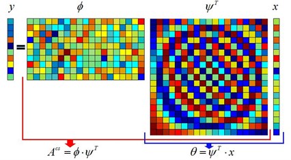
For the original signal, the first step is to transform the original signal to a sparse signal:

1

x = ψ \cdot θ, θ = ψ^{T} \cdot x,

where $x$ is $N$ ×1 vector; $ψ$ is sparse matrix, which is an orthogonal matrix of $N$ × $N$ ; $θ$ is sparse vector of $N$ ×1, which can be said $K$ -sparse if the vector contains only $K$ non-zero values $(K ≪ N)$ .

Then, it is the dimension reduction and can be represented as:

2

y = ϕ \cdot θ = ϕ \cdot ψ^{T} \cdot x = A^{C S} \cdot x,

where $ϕ$ is the observation matrix of $M \times N$ , $(M ≪ N)$ ; The compressed data $y$ is $M$ ×1 vector; $A^{C S}$ is the matrix of $M$ × $N$ $(A^{C S} = ϕ \cdot ψ^{T})$ .

The most important step of signal reconstruction is the recovery of $θ$ . The solution can be shown as follows:

3

m i n {‖θ‖}_{0} subject to y = ϕ \cdot θ .

Owing to the sparsity of $θ$ and the incoherence between $ψ$ and $ϕ$ , the vector $θ$ can be reconstructed with a high probability based on a reconstruction algorithm. After that, the original signal can be obtained by Eq. (1).

The dimension of the vector y is determined by:

4

M \geq C μ^{2} K l o g N,

where $C$ is a positive constant; and $μ$ is the correlation between $ψ$ and $ϕ$ , which can be represented as:

5

μ = \sqrt{N} \cdot \underset{i, j}{m a x} (|⟨ϕ_{i}, ψ_{j}⟩|),

where $ϕ$ is the random matrix, which is uncorrelated with any other matrix. The sparse matrices are usually the Fourier, DCT or wavelet matrices. In the following experiments, random matrices and Fourier matrices were used as observation matrices and sparse matrices, respectively.

2.2. Stochastic resonance

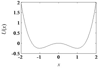
Stochastic resonance occurs in a nonlinear system with noise and periodic input signal, which can be described by the Langevin equation:

6

\dot{x} = - U^{'} (x) + s (t) + Γ (t),

where $s (t)$ is the periodic input signal; $Γ (t)$ denotes a Gaussian white noise with a zero-mean, which satisfies $⟨Γ (t)⟩ =$ 0 and $⟨Γ (t), Γ (0)⟩ \geq 2 D δ (t)$ , where $D$ is the noise intensity and $δ (t)$ is the unit impulse function; $U (x)$ is the traditional bistable potential function and is shown in Fig. 2. The barrier parameters $a$ and $b$ in $U (x)$ are positive real parameters:

7

U (x) = - \frac{a}{2} x^{2} + \frac{b}{4} x^{4}, a > 0, b > 0 .

According to Eq. (7), the barrier height is $Δ U = a^{2} / 4 b$ , and the steady state of the system is at:

x = \pm \sqrt{\frac{a}{b}} .

Then, Eq. (6) can be written as:

8

\dot{x} = a x - b x^{3} + s (t) + Γ (t) .

The periodic signal can be presented as $s (t) = A c o s 2 π F t$ . When the periodic signal and the noise are acting at the same time, the periodic signal will induce a periodic change to the system potential wells and synchronize the noise-induced switching.

Fig. 2The potential function Ux(a=b= 1)

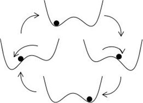
In the case that the amplitude of $s (t)$ is smaller than the critical value of the barrier height $A_{C} = \sqrt{4 a^{3} / 27 b}$ , the particles can cross from the original potential well to another potential well at Kramer’s rate $r_{k} = (a / \sqrt{2} π) e x p (- Δ U / D)$ . What’s more, the system output is switched between the two potential wells by the frequency $ω$ of the signal; the switching speed synchronizes the output signal with the weak periodic signal. When the transition rate matches the period of the input signal ( $2 / r_{k} = 1 / F$ ), the frequency $ω$ is equal to $F$ , the component of the frequency $F$ n the output $x (t)$ is enhanced. That is why stochastic resonance can strengthen the weak signal and improve the sparsity. The transition of particles between two potential wells is shown in Fig. 3.

Fig. 3The diagram of the transition between two potential wells of stochastic resonance

2.3. The proposed method

CS has been applied in many areas, such as nuclear magnetic resonance, image processing, etc. But CS is still little application in mechanical fault diagnosis field. The main problem is the poor sparsity of mechanical signal caused by the noise. Even worse, the useful fault feature information may be buried in noise, especially at the initial fault stages. As for the fault detection section, the traditional idea is to recover the whole signal from the compressed data, and then extract the fault characteristics from the whole signal, just like the workflow shown in Fig. 4(a). For the real vibration signals, this process is tedious and impossible because of the complex noise. So, there is a question, if it is possible to extract the faults directly from the compressed data rather than reconstruct the whole signal, just like the process shown in Fig. 4(b). The reconstruct methods of the signal are usually consisted of greedy pursuit’s algorithm, convex relaxation algorithm and combinatorial algorithm [21]. In this paper, Compressed Sampling Matching Pursuit (CSMP) algorithm is applied to reconstruct the signal, which is one kind of greedy pursuit’s algorithm. CSMP invokes the idea of iteratively to reconstruct the signal [22]. The current approximation induces a residual in each iteration. The samples are updated to reflect the current residual with the processing of algorithm. These samples construct a proxy for the residual, and it is useful to identify the large components in the residual. This step yields a tentative support for the next approximation. The samples to estimate the approximation on the support set. This process is repeated until we have found the recoverable energy in the signal. What’s more, CSMP needs to know the sparseness of the target signal in advance, which is very suitable for us to extract the fault feature frequency.

Fig. 4The compare of fault identification process between whole signal and compressed signal

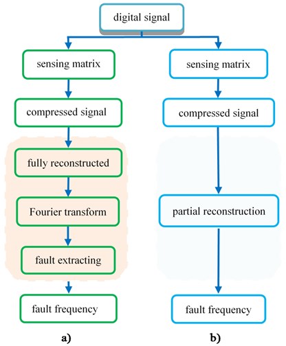
Table 1The steps for extracting fault feature frequency from compressed data

C S M P (φ, y, s)

Input: Sampling matrix

ϕ

, compresseddata

y

, sparsity level

s

;

Output: An

s

-saprse approximation

α

of the target signal

α^{0} \leftarrow 0

(Trivial initial approximation)

v \leftarrow y

(Current samples = input samples)

k \leftarrow 0

Repeat:

k \leftarrow k + 1

y \leftarrow ϕ^{*} \cdot v

(From signal proxy)

Ω \leftarrow s u p p (y_{2 k})

(Identify large components)

T \leftarrow Ω \cup s u p p (a^{k - 1})

(Merge supports)

b |_{T} \leftarrow ϕ_{T}^{- 1} \cdot y

(Signal estimation by least-squares)

b |_{T^{C}} \leftarrow 0

a^{k} \leftarrow b_{s}

(Prune to obtain next approximation)

v \leftarrow y - ϕ \cdot a^{k}

(Update current samples)

Until halting criterion true

The steps for extracting fault feature frequency from compressed data are shown in Table 1 (Algorithm 1. CSMP recovery algorithm).

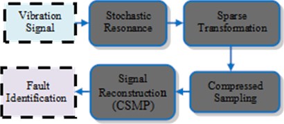
For the problem of weak feature identification under noise in mechanical fault diagnosis, the paper proposes a new method of weak feature identification based on CS and SR. In the method, we use stochastic resonance system to enhance the fault frequency and weaken the noise, so the sparseness of the signal gets better, and it is suitable to apply it to compressed sensing. First, we design a stochastic resonance system to process the vibration signal. Then, sparse transformation and compression sampling were taken. Finally, we use the CSMP algorithm to reconstruct the fault feature frequency from the compressed data. The flow chart of the method is shown in Fig. 5.

Fig. 5The workflow of the new method of the paper

3. Experiment and results

In this section, two experiments are performed with fault rings of roller element bearings to verify the effectiveness of the proposed method.

3.1. Inner ring Fault identification of a roller bearing

The original data of this case is come from the rolling bearing fault simulation platform of Case Western Reserve University [23]. As shown in Fig. 6, the test platform consists of a 2 hp motor (left), a torque transducer/encoder (center), a load motor (right). The test platform bearing comprises a drive end bearing and a fan end bearing. The bearing type of the motor housing used in the experiment is SKF6205, the bearing speed is $N =$ 1797 r/min, the sampling frequency is 12 kHz. The status is the inner ring fault and the other information is shown in Table 2.

Table 2The dimensions of the drive roller bearings

Inner diameter / mm	Outer diameter / mm	Pitch diameter $D$ / mm	Contact angle $β$ / (°)	Number of balls $n$	Balls diameter $d$ / mm
25.001	51.999	39.040	0	9.000	7.940

According to the formula:

9

f_{i} = \frac{n N}{120 d} (1 + \frac{d c o s β}{D}) .

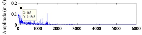
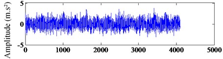
The theoretical value of the fault feature frequency of the inner ring $f_{i} =$ 162.18 Hz. Fig. 7 presents the waveform and spectra of bearing inner ring fault signal. Fig. 7(a) shows the waveform which exists a fault feature and the sparseness of the signal is poor. In Fig. 7(b), the spectral energy distributes over a wide frequency range and the fault feature frequency is submerged by other frequency signals. What’s more, the sparseness is poor too. So, it’s necessary to use SR to process the signal. After analyzing the fault feature frequency, we set the coefficients $a =$ 1, $b =$ 5, $D =$ 0.2, and we use this system to process the vibration signal.

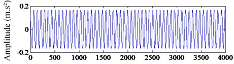
We use the proposed method to identify the fault signal. Fig. 8(a) shows the waveform after stochastic resonance. Fig. 8(b) shows the spectrum, which is also the sparse signal after sparse transformation. It’s clear that the fault feature frequency is enhanced, and the sparseness of the signal has been improved. It becomes feasible to use the CS to sample and then extract the fault feature frequency.

Fig. 6Rolling bearing test platform of West University

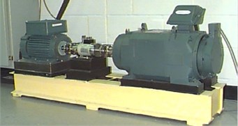
Fig. 7The waveform and spectrum of bearing inner ring fault signal: a) the waveform, b) the spectrum

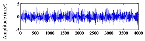
a) Data sequence

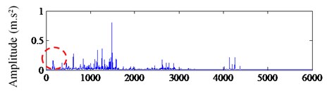
b) Frequency (Hz)

Fig. 8The waveform and spectrum after SR processing: a) the waveform after SR, b) the spectrum after SR

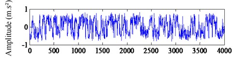
a) Data sequence

b) Frequency (Hz)

Fig. 9Compressed sampling signal

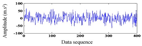
In this step, we select a compressible sampled signal section from that of Fig. 8 (a), which is presented in Fig. 9, with 400 samples compared to 4000 in Fig. 8. Here the sampling is not in a tradition way. Instead, it is obtained by multiplying the observation matrix, which is shown in Eq. (2). In this case, $ψ$ is a Fourier matrix of 4000×4000 and $ϕ$ is a random matrix of 400×4000. Next, it is time to extract the fault feature frequency.

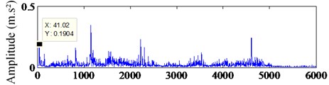
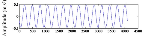
In Fig. 10, the extracted signal is shown. Fig. 10(a) shows the sparse signal, which is recovered from the compressed data using CSMP algorithm. It is clear that the signal only contains the fault feature frequency component of 162 Hz. Fig. 10(b) shows waveform of extracted signal. This experiment presents that the proposed method is feasible.

Fig. 10The extracted fault feature signal: a) the frequency spectrum of extracted signal, b) the waveform of extracted signal

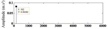
a) Frequency (Hz)

b) Data sequence

3.2. Outer ring fault identification of roller bearing

The experimental data is come from the middle speed shaft outer ring of rotating machinery fault diagnosis test platform, which is shown in Fig. 11. In this case, the bearing model is ER-16K, and we select the data of working condition 29. The measuring point is the middle speed end near the motor end. The speed ratio and load ratio are 80 %. The fault feature frequency characteristic of the middle speed shaft of the working condition 29 is 41.435 Hz. In the experiment, the maximum speed of the motor is 3000 rpm, the maximum frequency is 50 Hz, the motor speed is calculated: 3000×80 % = 2400, and the sampling frequency is 12 kHz. In Fig. 12, the bearing outer ring fault signal is presented. Fig. 12(a) shows the waveform and Fig. 12(b) shows the spectrum of the vibration signal. It is obvious that fault feature information is submerged in the noise and there is no way to identify the fault feature. What’s more, the sparseness of the signal is poor not only in time domain but also in frequency domain. So, it is necessary to use stochastic resonance to process the vibration signal. In this case, we set the coefficients $a =$ 1, $b =$ 5, $D =$ 0.2.

Fig. 11The test platform

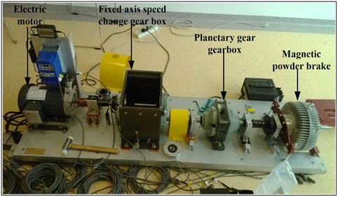
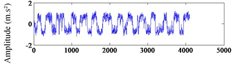
Fig. 13(a) shows the waveform after stochastic resonance while Fig. 13(b) presents the spectrum. It’s clear that the fault feature frequency is enhanced, and the sparseness of the signal has been improved. It becomes feasible to use the CS to sample and then extract the fault feature frequency.

Fig. 12The waveform and spectra of bearing outer ring fault signal: a) the waveform of original signal, b) the spectrum of original signal

a) Data sequence

b) Frequency (Hz)

Fig. 13The waveform and spectra of the signal after stochastic resonance processing: a) the output waveform of SR, b) the spectrum of SR

a) Data sequence

b) Frequency (Hz)

Same as case 1, the compressed data $y$ is shown in Fig. 14, with 400 sample points compared to 4000 in Fig. 13. It is obtained by multiplying the observation matrix, which is shown in Eq. (2). In this case, $ψ$ is a Fourier matrix of 4000×4000 and $ϕ$ is a random matrix of 400×4000.

Fig. 14Compressed sampling for fault diagnosis

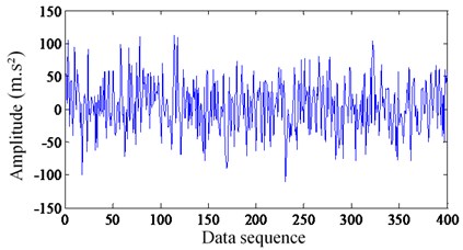
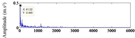
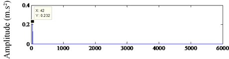
Fig. 15 shows the extracted signal. Fig. 15(a) shows the sparse signal, which is recovered from the compressed data using CSMP algorithm. Fig. 15(b) presents the waveform of extracted signal. It is clear that the signal only contains frequency of 42 Hz, which is very close to the fault feature frequency of 41.435 Hz. This case presents that the proposed method is feasible.

Fig. 15The extracted signal of fault feature frequency: a) the frequency spectrum of extracted signal, b) the waveform of extracted signal

a) Frequency (Hz)

b) Data sequence

4. Conclusions

In this paper, a weak fault identification method is proposed based on CS theory and SR. The machine fault vibration signals are pretreated by stochastic resonance. By this way, the fault signal drowned by noise is amplified and the sparseness of the signals is enhanced, which make it possible to apply compressed sensing. One most outstanding advantage of the method is to extract the mechanical fault feature directly from the compressed data without recovering completely, which reduces the dimensionality of the measurement data and the complexity of algorithm. Another advantage of the method is to defect fault feature directly from far fewer measurements than the Shannon sampling theory requires. The effectiveness of the method has been validated by two experiments.

References

Liu J., Shao Y. Overview of dynamic modelling and analysis of rolling element bearings with localized and distributed faults. Nonlinear Dynamics, Vol. 93, 2018, p. 1765-1798.

Publisher
Naiquan S. U., Jianbin X., Qinghua Z., et al. Research methods of the rotating machinery fault diagnosis. Machine Tool and Hydraulics, Vol. 46, Issue 7, 2018, p. 133-139.

Search CrossRef
Jianqing Y. U., Guanjian Z., Shikun X., et al. The summary of signal processing technology in fault diagnosis for rotating machinery. Machine Tool and Hydraulics, Vol. 39, Issue 24, 2011, p. 107-110.

Search CrossRef
Ferguson D., Catterson V. Big data techniques for wind turbine condition monitoring. European Wind Energy Association Annual Event, 2014.

Search CrossRef
Donoho D. L. Compressed sensing. IEEE Transactions on Information Theory, Vol. 52, Issue 4, 2006, p. 1289-1306.

Publisher
Candes E. J., Tao T. Near-optimal signal recovery from random projections: universal encoding strategies. IEEE Transactions on Information Theory, Vol. 52, Issue 12, 2006, p. 5406-5425.

Publisher
Candè E. J., Wakin M. B. An introduction to compressive sampling. IEEE Signal Processing Magazine, Vol. 25, Issue 2, 2008, p. 21-30.

Publisher
Wang H., Ke Y., Luo G., et al. Compressed sensing of roller bearing fault based on multiple down-sampling strategy. Measurement Science and Technology, Vol. 27, Issue 2, 2016, p. 025009.

Publisher
Du Z., Chen X., Zhang H. Feature identification with compressive measurements for machine fault diagnosis. Instrumentation and Measurement Technology Conference, 2015.

Search CrossRef
Tang G., Hou W., Wang H., et al. Compressive sensing of roller bearing faults via harmonic detection from under-sampled vibration signals. Sensors, Vol. 15, Issue 10, 2015, p. 25648.

Publisher
Yuan H., Lu C. Rolling bearing fault diagnosis under fluctuant conditions based on compressed sensing. Structural Control and Health Monitoring, Vol. 24, Issue 5, 2017, p. e1918.

Publisher
Tang G., Yang Q., Wang H. Q., et al. Sparse classification of rotating machinery faults based on compressive sensing strategy. Mechatronics, Vol. 31, 2015, p. 60-67.

Publisher
Benzi R., Sutera A., Vulpiani A. The mechanism of stochastic resonance. Journal of Physics A: Mathematical and General, Vol. 14, Issue 11, 1999, p. L453.

Publisher
Mcdonnell M. D., Abbott D. What is stochastic resonance? Definitions, misconceptions, debates, and its relevance to biology. PLOS Computational Biology, Vol. 5, Issue 5, 2009, p. e1000348.

Publisher
Benzi R. Stochastic resonance: from climate to biology. Nonlinear Processes in Geophysics, Vol. 17, Issue 5, 2007, p. 431-441.

Publisher
Gammaitoni L., Hanggi P., Jung P., et al. Stochastic resonance: a remarkable idea that changed our perception of noise. European Physical Journal B, Vol. 69, Issue 1, 2009, p. 1-3.

Publisher
Han D., Li P., An S., et al. Multi-frequency weak signal detection based on wavelet transform and parameter compensation band-pass multi-stable stochastic resonance. Mechanical Systems and Signal Processing, Vol. 70, Issue 71, 2016, p. 995-1010.

Publisher
Li J., Chen X., He Z. Multi-stable stochastic resonance and its application research on mechanical fault diagnosis. Journal of Sound and Vibration, Vol. 332, Issue 22, 2013, p. 5999-6015.

Publisher
Qin Y., Tao Y., He Y., et al. Adaptive bistable stochastic resonance and its application in mechanical fault feature extraction. Journal of Sound and Vibration, Vol. 333, Issue 26, 2014, p. 7386-7400.

Publisher
Zhang X., Hu N., Hu L., et al. Enhanced detection of bearing faults based in signal cepstrum pre-whitening and stochastic resonance. Journal of Mechanical Engineering, Vol. 48, Issue 23, 2012, p. 83-89.

Publisher
Candes E. J., Romberg J. Errata for quantitative robust uncertainty principles and optimally sparse decompositions. Foundations of Computational Mathematics, Vol. 7, Issue 4, 2007, p. 529-531.

Publisher
Needell D., Tropp J. A. CoSaMP: Iterative signal recovery from incomplete and inaccurate samples. Applied & Computational Harmonic Analysis, Vol. 26, Issue 3, 2009, p. 301-321.

Publisher
Case Western Reserve University Bearing Data Center Website. http://csegroups.case.edu/bearingdatacenter/home.

Search CrossRef

Cited by

Fault Diagnosis Method of Planetary Gearbox Based on Compressed Sensing and Transfer Learning

Huajun Bai | Hao Yan | Xianbiao Zhan | Liang Wen | Xisheng Jia

(2022)

Weak fault signature identification of rolling bearings based on improved adaptive compressed sensing method

Jianyu Zhang | Guofeng Wang

(2021)

Bearing Fault Diagnosis Based on State-Space Principal Component Tracking Filter Algorithm

Tangshao Duan | Zhiqiang Liao | Taifu Li | Haihong Tang | Peng Chen

(2021)

2020 IEEE 16th International Conference on Control & Automation (ICCA)

Zhenjin Shi | Yueyang Li | Shuai Liu

(2020)

About this article

Received

14 August 2018

Accepted

25 December 2018

Published

15 May 2019

SUBJECTS

Fault diagnosis based on vibration signal analysis

DOI

https://doi.org/10.21595/jve.2018.20140

Keywords

rotating machinery

weak fault diagnosis

feature extraction

compressed sensing

stochastic resonance

Acknowledgements

This work was supported by the National Natural Science Foundation of China (Grant No. 51475407, 51605419), China Postdoctoral Science Foundation (Grant No. 2016M600193) and Training Fund of Talent Project in Hebei Province (Grant No. A2016002018).

This is an open access article distributed under the Creative Commons Attribution License, which permits unrestricted use, distribution, and reproduction in any medium, provided the original work is properly cited.

Previous article in issue Previous Next article in issue Next

Review article

2021 11 26

Fault diagnosis and health management of bearings in rotating equipment based on vibration analysis – a review

Adnan Althubaiti, Faris Elasha, Joao Amaral Teixeira

Research article

2021 06 22

Periodic non-sinusoidal time-delay stochastic resonance weak fault diagnosis method and its application

Zhixing Li, Huiru Bao, Songjiu Han

Research article

2019 09 30

Bearing fault diagnosis based on feature extraction of empirical wavelet transform (EWT) and fuzzy logic system (FLS) under variable operating conditions

Fawzi Gougam, Chemseddine Rahmoune, Djamel Benazzouz, Boualem Merainani

Research article

2017 11 15

Feature reconstruction based on t-SNE: an approach for fault diagnosis of rotating machinery

Jiayu Chen, Dong Zhou, Chuan Lyu, Chen Lu

P. Shi, X. Ma, and D. Han, “A weak fault diagnosis method for rotating machinery based on compressed sensing and stochastic resonance,” Journal of Vibroengineering, Vol. 21, No. 3, pp. 654–664, May 2019, https://doi.org/10.21595/jve.2018.20140

Copy Extrica

Copied to clipboard!

TY  - JOUR
DO  - 10.21595/jve.2018.20140
UR  - https://doi.org/10.21595/jve.2018.20140
TI  - A weak fault diagnosis method for rotating machinery based on compressed sensing and stochastic resonance
T2  - Journal of Vibroengineering
AU  - Shi, Peiming
AU  - Ma, Xiaojie
AU  - Han, Dongying
PY  - 2019
DA  - 2019/05/15
PB  - JVE International Ltd.
SP  - 654-664
IS  - 3
VL  - 21
SN  - 1392-8716
SN  - 2538-8460
ER  - 

Copy Ris

Copied to clipboard!

@article{Shi_2019,
	doi = {10.21595/jve.2018.20140},
	url = {https://doi.org/10.21595/jve.2018.20140},
	year = 2019,
	month = {may},
	publisher = {{JVE} International Ltd.},
	volume = {21},
	number = {3},
	pages = {654--664},
	author = {Peiming Shi and Xiaojie Ma and Dongying Han},
	title = {A weak fault diagnosis method for rotating machinery based on compressed sensing and stochastic resonance},
	journal = {Journal of Vibroengineering}
}

Copy Bibtex

Copied to clipboard!

[1]P. Shi, X. Ma, and D. Han, “A weak fault diagnosis method for rotating machinery based on compressed sensing and stochastic resonance,” Journal of Vibroengineering, vol. 21, no. 3, pp. 654–664, May 2019, doi: 10.21595/jve.2018.20140.

Copy IEEE

Copied to clipboard!

Shi, Peiming, Xiaojie Ma, and Dongying Han. “A Weak Fault Diagnosis Method for Rotating Machinery Based on Compressed Sensing and Stochastic Resonance.” Journal of Vibroengineering 21, no. 3 (May 15, 2019): 654–64. https://doi.org/10.21595/jve.2018.20140.

Copy Chicago

Copied to clipboard!

A weak fault diagnosis method for rotating machinery based on compressed sensing and stochastic resonance

Abstract

1. Introduction

2. The method for weak feature identification

2.1. Compressed sensing

2.2. Stochastic resonance

2.3. The proposed method

3. Experiment and results

3.1. Inner ring Fault identification of a roller bearing

3.2. Outer ring fault identification of roller bearing

4. Conclusions

References

Cited by

About this article

Related Articles