Experimental and numerical study of the behavior of shallow rectangular tunnels

Hassanzadeh, Mehran; Hajialilue Bonab, Masoud; Javadi, Akbar A.

doi:10.21595/jve.2018.19308

Journal of Vibroengineering

Browse Journal

Submit article

Published: 30 June 2018

Check for updates

Experimental and numerical study of the behavior of shallow rectangular tunnels

Mehran Hassanzadeh¹

Masoud Hajialilue Bonab²

Akbar A. Javadi³

^{1, 2}Faculty of Civil Engineering, University of Tabriz, Tabriz, Iran

³Department of Engineering, University of Exeter, Exeter, UK

Corresponding Author:

Mehran Hassanzadeh

Cite the article Download PDF

Downloads 2095

WoS Core Citations 6

CrossRef Citations 6

Abstract

The behavior of an underground structure under dynamic loading is affected by many factors such as shape, depth and stiffness of the structure as well as the frequency content of the input motion. Scarcity of experimental/field investigations precludes proper understanding of these parameters’ effects on the seismic behavior of aforementioned structures. In this study, the effects of input motion along with structural stiffness properties on seismic behavior of rectangular tunnels are investigated. Three reduced-scale 1 g shaking table models were constructed in 1/48 scale. Tests were carried out in the shaking table facility at the University of Tabriz on model tunnels of the rectangular section of the shallow Tabriz subway tunnel, using input motions of different amplitudes and frequencies. In addition, a numerical study was done using the coupled scaled boundary finite element-finite element (SBFE-FE) method. A good agreement between the numerical model and the results of the experimental test was achieved. Using the shaking table test, the accelerations and bending moments of the tunnel lining were measured. The results show that tunnel lining stiffness affects the acceleration response of the ground. A parametric study by the numerical approach was presented and effects of the variation of elastic modulus and mass density of the soil were evaluated.

1. Introduction

Modern cities inherit common problems like sewage waste, mass transportation, water transport and material supply. In recent decades, these problems have been commonly addressed using underground facilities. In many cities located in seismically active areas, such underground facilities face the risk of damage due to earthquake. Some underground structures have experienced significant damage in recent large earthquakes, including the 1995 Kobe earthquake in Japan, the 1999 Chi-Chi earthquake in Taiwan and the 1999 Kocaeli earthquake in Turkey [1]. The behavior of tunnels under dynamic loading is affected by the depth of the tunnel below the ground surface, type of soil or rock surrounding the tunnel, maximum ground acceleration, intensity of the earthquake, distance to the earthquake epicenter and type of tunnel lining. Considering the importance of the subject, many researchers have conducted experimental and numerical studies on different aspects of seismic behavior of underground structures. Several numerical studies have been carried out by many researchers, such as Hashash et al., [2]; Huo et al., [3]; Anastasopoulos et al., [4, 5]; Amorosi and Boldini, [6]; Kontoe et al., [7, 8]; Baziar et al., [9]; Bilotta et al., [10]; to study the behavior of underground structures under dynamic loading. Also, a number of experimental studies have been carried out in recent years. Using centrifuge facilities at Cambridge University, Lanzano et al. [11] assessed the effect of a circular tunnel on the acceleration response of nearby ground. The effects of the tunnel depth and soil density were studied in their experiments. Pitilakis et al. [12] carried out a series of tests in order to validate numerical simulations of soil-structure interaction effects using a centrifuge model structure and non-liquefiable soil. Guoxing et al. [13] performed shaking table tests to investigate the damage mechanisms of a subway structure in soft soil under strong ground motions. Their results provided insight into how the characteristics of strong ground motion might influence the structure. They presented a simplified analysis method to quantitatively evaluate the damage of subway structures in soft soil. Penzien [14] reported that ovaling and racking of tunnel lining are the most critical sources of damage to tunnel structures. Damage is reported to be increasing as the duration of the earthquake increases, because repeated load cycles cause fatigue in the tunnel lining [1]. Cilingir and Madabhushi [15] performed an investigation into the effects of input motion characteristics such as frequency, amplitude and duration on the dynamic behavior of circular and square tunnels under vertically propagating transverse shear waves. The results showed that both circular and square tunnels suffer changes in earth pressures and lining forces in the first few cycles after the start of the earthquake and quickly reach to an equilibrium stage where both lining forces and earth pressures oscillate around a mean value until the end of the earthquake. Rabeti and Baziar [16] investigated the effect of circular tunnel of Tehran subway on the ground motion amplification pattern by means of shaking table and numerical modeling. Tsinidis et al., [17] studied the seismic earth pressures imposed on tunnel side-walls, seismic shear stresses around the structure, and complex deformation modes of tunnels mobilized during shaking using dynamic centrifuge testing and numerical analysis. The scaled boundary finite element method is a semi analytical method which couples the advantages of the two mostly used finite element (FE) and boundary element methods [18]. In the scaled boundary finite element method (SBFEM), by using a scale center (SC) and two dimensionless local coordinates ( $η$ , $ξ$ ) (for two-dimensional (2D) problems) the governing equations can be transformed to a new coordinate system. Different numerical investigations were investigated using the SBFEM. For seismic analyses, Junyi et al., [19] proposed a free field input model based on the coupled scaled boundary finite element-finite element (SBFE-FE) method in time domain. Genes and Kocak [20] used the SBFE-FE method to analyze seismic soil structure interaction problems. Nonlinear seismic investigation was carried out in [21] to predict building responses to earthquake loading. Seiphoori et al. [22] used the SBFE-FE method for three-dimensional analysis of concrete rock fill dams. Bazyar and Basirat [23] detailed the formulation of the SBFEM to investigate seismic problems. Tohidvand and Hajialilue-bonab [24] carried out a seismic soil-structure interaction analysis using the coupled scaled boundary spectral element-spectral element method.

Tabriz is a highly-populated city, located in a seismically active region in the north-west of Iran. The seismic impact of possible earthquakes has been an important part of the feasibility study and design of the Tabriz subway. In this paper, experimental and numerical study were performed to better understand the effects of seismic loading on the behavior of underground rectangular tunnels. In this regard, small scaled 1g shaking table tests with two rectangular tunnel sections under different loading conditions were carried out. The effects of input motion on tunnel behavior and acceleration amplification within the shear box were investigated. The soil-tunnel flexibility ratio was determined using the experimental results. In what follows the used shaking table is described together with the sample preparation and instrumentation procedure and the loading characteristics. A brief description of the SBFEM is presented and the results of the tests and numerical investigations are then presented and discussed.

2. Shaking table testing

2.1. Shaking table facility of University of Tabriz

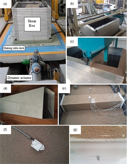
The experiments were carried out using the 1D shaking table in the geotechnical laboratory of the University of Tabriz. Input motions were applied at the base of the model through an actuator, which is capable of imposing time history and sinusoidal excitations up to 6 tons of maximum payload mass. The deck size of the shaking table is 200 cm in width and 300 cm in length. A laminar shear box container was employed to mount the models, having inner dimensions 132 cm in length, 86 cm in width and 84 cm in depth and consisting of horizontal layers made from aluminum tubes. The box was designed in order to simulate free field behavior of ground, thus minimizing the boundary effects due to soil-container interactions. The shaking table and soil shear box are shown in Fig. 1.

Fig. 1a) University of Tabriz shaking Table, b) shear box and sand pluviation device, c) sand pouring, d) aluminum tunnel model, e) model preparation, f) 0.01 g accelerometer, g) Teflon plate and EPE foam

a) University of Tabriz shaking Table, b) shear box and sand pluviation device, c) sand pouring, d) aluminum tunnel model, e) model preparation, f) 0.01 g accelerometer, g) Teflon plate and EPE foam

2.2. Soil and model tunnels

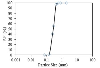
The soil used was sand obtained from Goumtapa (an area near Tabriz city). The physical properties of the sand are presented in Table 1, and the particle size distribution curve is depicted in Fig. 2. The soil can be classified as SP according to the Unified Soil Classification System (USCS).

Table 1Physical and mechanical properties of Ghomtapa sand

$γ_{m a x}$ (kN/m³)	$G_{s}$	$d_{50}$ (mm)	$φ$ (◦)	$φ_{c r i t}$ (◦)
17.38	2.635	0.175	33	31

Fig. 2Particle size distribution of Ghoumtapa sand

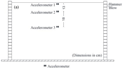
The concrete tunnel section of Tabriz subway was scaled to a model tunnel made of aluminum sheet, 1.5mm in thickness. For this purpose, scaling laws proposed by Iai [25] for 1g shaking table tests and tunnel stiffness ratios were employed Eq. (1). The soil density scale factor, $λ_{ρ}$ was assumed to be unity. In order to determine the strain scale factor ( $λ_{ε}$ ) in Eq. (2), a hammer test was performed on the shear box utilizing three accelerometers to obtain the soil shear wave velocity:

1

\frac{{(E I)}_{p}}{{(E I)}_{m}} = \frac{λ^{4} λ_{ρ}}{λ_{ε}},

2

λ_{ε} = \frac{λ}{{(\frac{{(V_{s})}_{p}}{{(V_{s})}_{m}})}^{2}} .

In the above equations ${(E I)}_{p}$ and ${(E I)}_{m}$ are prototype and model tunnel stiffness; ${(V s)}_{p}$ and ${(V s)}_{m}$ are prototype and model soil shear wave velocities; $λ$ , $λ_{ε}$ and $λ_{ρ}$ are scale factors for length, strain and soil density, respectively. The soil shear wave velocities for intervals between the accelerometers 1 and 2, and 2 and 3 were determined as 43 m/s and 90 m/s, respectively.

In this study, the shear wave velocity of 45 m/s was adopted for the model sand, which is reasonable for a soil with low confining pressure, whereas, the shear velocity of the prototype soil is 375 m/s. Therefore, the scaling factor is derived by combining Eqs. (1) and (2) resulting in $λ =$ 48. The similitude ratios of the model structure and soil are listed in Table 2. Scaling the prototype tunnel section into the model tunnel, results in 12.5 cm height and 17.5 cm width as shown in Fig. 3.

Table 2Iai similitude ratios [18]

Length	$λ$
Density	$λ_{ρ}$
Time	${(λ λ_{ε})}^{0.5}$
Bulk Modulus	$λ λ_{ρ} / λ_{ε}$
Acceleration	1
Velocity	${(λ λ_{ε})}^{0.5}$
Displacement	$λ λ_{ε}$
Stress	$λ λ_{ρ}$
Strain	$λ_{ε}$
Flexural Rigidity	$λ^{4} λ_{ρ} / λ_{ε}$

Also, another model tunnel section with thickness of 1mm was made of aluminum sheet for the purpose of comparison, with identical height and width to the previously mentioned section. The tests that were performed with 1.5mm tunnel section are indexed as RT and those with 1mm section are indexed as FT. To increase the interaction between soil and model tunnels, their surfaces were covered and glued with a thin layer of model sand. The model tunnel is shown in Fig. 1(d) and (e).

2.3. Model preparation and instrumentation

The sand was poured in the shear box using an automatic sand pluviation device to maintain the density of sand identical for all tests. This device moves automatically back and forth over the shear box, generating a curtain of sand from its bottom slot (Fig. 1(c)). The soil relative density is controlled by the height and amount of sand dropped from the slot. The pluviation device was configured in a way that it produced relative density of 65 % inside the shear box. During the pouring process, the tunnel and accelerometers were positioned in the shear box (Fig. 1(d) and 1(e)). In order to avoid any interaction between the tunnel and the container, the model tunnels were made shorter than the shear box width. A thin sheet of aluminum foil EPE foam and a Teflon plate was used to cover tunnel ends. As shown in Fig. 1(g), the aluminum foil is in contact with the Teflon plate, thus eliminating the friction induced by tunnel deformations during shaking.

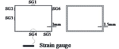
Four accelerometers with precision of 0.01 g were introduced within the soil to examine the acceleration response of the soil and the tunnel models (Fig. 3). Accelerometers were placed in a vertical array centered within the shear box. To measure the bending moments in the model tunnel, six resistance strain gauges were glued on the outer face of the tunnel. Three of them measured the bending moments near the model corners and the other three recorded bending moments at the middle of the roof slab. The strain gauge configuration is shown in Fig. 4.

Fig. 3Model accelerometer layout

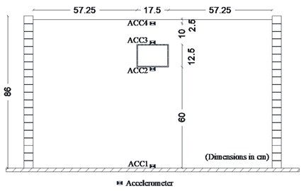
Fig. 4Model tunnel strain gauge configuration

Three types of scaled models were prepared within the shear box, with 1.5 mm model tunnel, 1 mm model tunnel and without tunnel indicated as RT, FT and FF respectively.

2.4. Loading characteristics

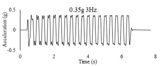
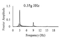
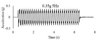
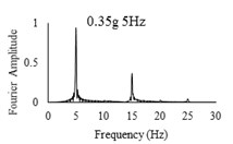
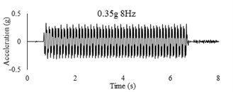
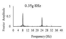
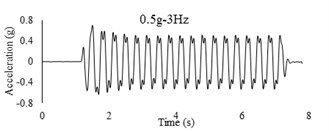
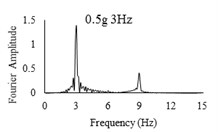
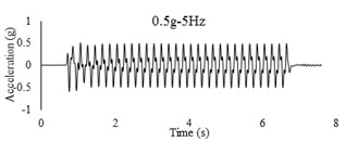
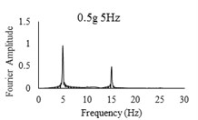
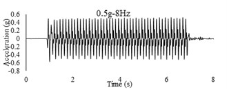
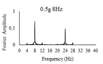
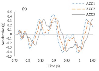
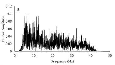
Three sets of artificial motions were produced to study the dynamic response of the soil and the model tunnel. For the first set of motions, a series of harmonic waves, with high acceleration magnitudes and different frequencies were applied at the shear box base. The second set of motions contained irregular broadband frequency waves. Similarly, the third set of motions, were created with same frequency content of the second motion set but with lower acceleration levels. The frequency bandwidth for irregular motions was set to 0.1-50 Hz. Fig. 5 illustrates the acceleration time histories and Fourier spectra of the harmonic input motions recorded by ACC1 accelerometer placed at the base of the soil deposit.

It is worth noting that the differences of frequency and amplitude for the input motions for all tests were negligible, verifying the repeatability of the input motions. The acceleration and strain gauge recordings were acquired during shaking at a sampling frequency rate of 100 Hz by means of NI 9205 data acquisition system. A fourth-order Butterworth band-pass filter with low and high cut-off frequency at respectively 0.5 and 50 Hz was applied to the time histories of the recorded acceleration and tunnel bending moments.

Fig. 5Time history and frequency content of input motions

3. A brief description of the scaled boundary finite element method

The scaled boundary finite element method (SBFEM) is a relatively novel, semi analytical approach, which can be applied to model bounded and unbounded mediums accurately. This method has four coefficient matrices ( $E^{0}$ , $E^{1}$ , $E^{2}$ , and $M^{0}$ ), where $E^{0}$ is a positive definite, symmetric matrix and can be calculated using Eq. (3). $E^{1}$ is a non-symmetric matrix, which contains both shape functions and their derivatives. $E^{1}$ may be calculated using Eq. (4). $E^{2}$ is another symmetric matrix and can be derived using Eq. (5). $M^{0}$ can be considered as the mass matrix of unbounded media and Eq. (6) can be used to construct this matrix [18]:

3

[E^{0}] = \int_{- 1}^{+ 1} [B^{1}]^{T} [D] [B^{1}] | J | d η,

4

[E^{1}] = \int_{- 1}^{+ 1} [B^{2}]^{T} [D] [B^{1}] | J | d η,

5

[E^{2}] = \int_{- 1}^{+ 1} [B^{2}]^{T} [D] [B^{2}] | J | d η,

6

[M^{0}] = \int_{- 1}^{1} [N (η)]^{T} ρ [N (η)] |J| d η .

In these equations, [ $D$ ] and [ $ρ$ ] are elasticity and density matrices respectively, and [ $B^{1}$ ] contains shape functions and [ $B^{2}$ ] contains derivatives of shape functions [18].

For dynamic or seismic loading cases, the equation of motion can be written as:

7

[\begin{array}{l} k_{i i} & k_{i Γ} \\ k_{Γ i} & k_{Γ Γ} \end{array}] [\begin{array}{l} u_{i} (t) \\ u_{Γ} (t) \end{array}] + [\begin{array}{l} C_{i i} & C_{i Γ} \\ C_{Γ i} & C_{Γ Γ} \end{array}] [\begin{array}{l} v_{i} (t) \\ v_{Γ} (t) \end{array}] + [\begin{array}{l} M_{i i} & M_{i Γ} \\ M_{Γ i} & M_{Γ Γ} + γ Δ t M_{0}^{\infty} \end{array}] [\begin{array}{l} a_{i} (t) \\ a_{Γ} (t) \end{array}] = [\begin{matrix} p_{i} (t) \\ p_{Γ} (t) - r_{Γ} (t) \end{matrix}],

where [ $M$ ], [ $C$ ] and [ $K$ ] are mass, damping and stiffness matrices respectively and $\{a\}$ , $\{v\}$ and $\{u\}$ are acceleration, velocity and displacement vectors. The subscript $Γ$ indicates degrees of freedom of the nodes on the near and far field interface. The subscript ( $i$ ) denotes degrees of freedom on the remaining nodes of the structure. In this equation, $\{r_{Γ}\}$ is the interaction force vector and for seismic loading case can be calculated as:

8

r (t) = \int_{0}^{t} M^{\infty} (t - τ) \{a (τ) - a_{g} (τ)\} d τ,

where $M^{\infty} (t)$ is the acceleration unit impulse response matrix and $a_{g}$ is theseismic acceleration.

4. Results and discussion

4.1. Hammer test

Prior to the loading procedure with the shaking table, a hammer blow test was performed manually on the soil column. Soil was poured inside the shear box (following the same steps that were used for the model tests) on the shaking table using the automatic pluviation device with placing a vertical array of only three accelerometers within the soil. A plastic hammer was then used to create excitation in the first accelerometer placed at the top of the soil column. Fig. 6(a) and (b) show the arrangement of the accelerometers and the time history of waves passing through them. The difference between arrival times of shear waves to each accelerometer was determined. The shear wave velocity of the soil within the shear box was obtained in intervals between the accelerometers with distance to time ratios. As mentioned earlier, the shear wave velocities for above and below intervals were 43 and 90 m/s, respectively.

Fig. 6a) Shear box configuration for hammer test, b) transmitted wave time history during hammer test

4.2. Soil and tunnel horizontal acceleration

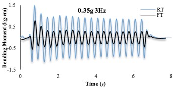
Results of the acceleration time history for observation point of ACC4, ACC3 and ACC2 in the RT model are shown in Fig. 7. This figure indicates that a good agreement between the numerical and experimental approaches are obtained.

Fig. 7Comparison between numerical and shaking table tests records in RT model for 0.35 g-3 Hz input motion

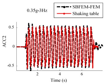
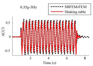
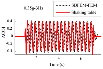
Fig. 8Peak accelerations for three state of tests, FT, RT and FF

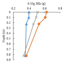
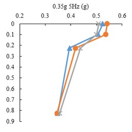
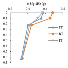
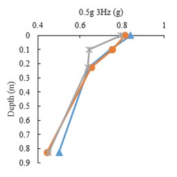
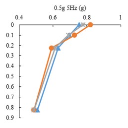
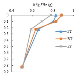
The peak acceleration profiles with depth along the accelerometer array in the three model states, FF, FT and RT, for harmonic input motions are presented in Fig. 8. The point mark at zero depth indicates the ACC4 accelerometer. It is shown that the peak accelerations decrease with depth in all tests. However, there is a difference in acceleration increment of the tunnel and free field, where the tunnel roof accelerometer shows higher amplification with respect to free field at the same burial depth. This indicates tunnel’s linear behavior as opposed to soil’s non-linear behavior.

The peak acceleration differences between ACC2 and ACC3 (tunnel base and roof) with respect to input frequency is depicted in Fig. 9. The amplification is the highest in the 1.5 mm model tunnel test and is higher in the 1 mm tunnel test than the free field test. The differences increase with higher input frequencies.

Fig. 9Acceleration discrepancy of tunnel base and roof a) 0.35 g, b) 0.5 g

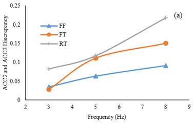
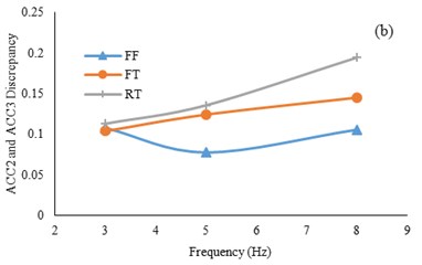
Fig. 10Irregular broadband input motions and transfer functions with a) low acceleration amplitude and b) high acceleration amplitude

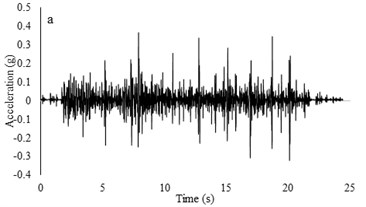
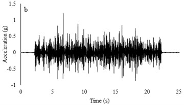
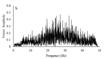
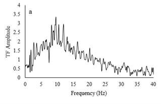
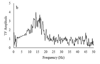
Two types of irregular broadband frequency input motions with low and high acceleration contents were used to evaluate the model resonant frequency. The low intensity motion has different spectral density than the motion with higher acceleration amplitudes. Transfer functions were calculated by dividing the cross spectral density of acceleration traces by the power spectral density of the input signals. Due to similarity between outputs for all models for each set of motions, only the input motions for the RT model are presented. Frequencies around 9-10 Hz are detected to be resonant frequency for lower amplitude motion but for higher acceleration content motion, resonant frequency has shifted to 14-16 Hz. The input motions and transfer functions for the RT model are illustrated in Fig. 10.

4.3. Bending moment of tunnel lining

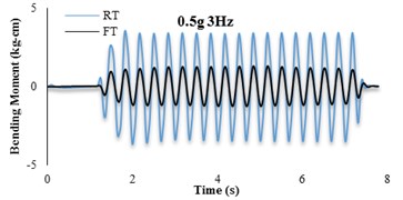
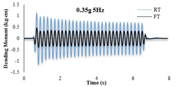
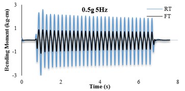
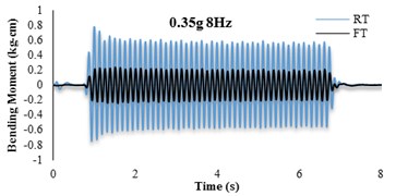
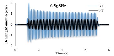
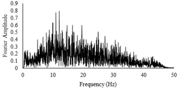
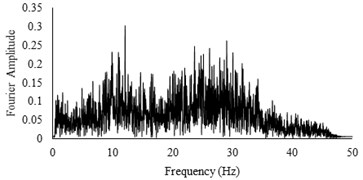
The bending moment-time histories for SG6 strain gauge are presented in Fig. 11. The dynamic bending moments at the corners of the tunnels were found to be larger than those in the middle of the slabs and the recorded values for the RT model are found to be larger than FT models. For further insight, the bending moment frequency domain of irregular input motion is depicted in Fig. 12. By comparison with Fig. 11(b) it is seen that the tunnel bending moment response for frequencies between 10-12 Hz is the highest. This confirms an adherence between soil and tunnel deformations.

Fig. 11Bending moment time histories of SG6

4.4. Soil-tunnel flexibility ratios

Soil-Tunnel flexibility ratio for FT and RT models were computed using the following equation (Wang [19]):

9

F = \frac{G_{m}}{24} (\frac{H^{2} W + H W^{2}}{E I}),

where $G_{m}$ is the soil shear modulus, $H$ is the tunnel height, $W$ is the tunnel width and EI is the tunnel transversal stiffness. The flexibility ratios for the RT and FT models were calculated as 355 and 1200, respectively. The racking ratios based on soil and structure distortions were derived by double integration of acceleration time histories using the following equation:

10

R = \frac{Δ_{s t r u c t u r e}}{Δ_{f f}},

where $Δ_{s t r u c t u r e}$ is the difference between ACC3 and ACC2 accelerometers in RT and FT models whereas $Δ_{f f}$ is the difference between ACC3 and ACC2 accelerometers in FF model. The racking ratios are shown in Table 3. Due to off phase deformation between ACC2 and ACC3 time histories in 0.35 g, 3 Hz loading, racking ratios were not defined. The results indicate that both tunnels behave as a flexible structure with respect to the surrounding soil, as the structural distortions are increased compared to the soil.

Fig. 12Bending moment frequency domain of SG6 strain gauge for irregular input motion with high acceleration amplitude

a) RT

b) FT

Table 3Racking ratios for RT and FT models

Input motion	FT	RT
0.35 g 3 Hz	–	–
0.35 g 5 Hz	3.3	4.54
0.35 g 8 Hz	4.02	3.06
0.5 g 3 Hz	1.3	1.33
0.5 g 5 Hz	2.07	2.03
0.5 g 8 Hz	1.89	1.19

4.5. Numerical parametric study

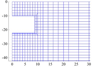
To evaluate the effects of different parameters on the tunnel-soil response, a numerical study, employing the coupled scaled boundary finite element-finite element (SBFE-FE) method is carried out. Fig. 13 shows the used mesh in this study. Given the symmetry, only half of the system has been modeled.

Fig. 13The SBFE-FE mesh of the tunnel-soil model

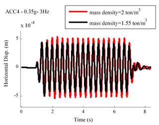
The variation effects regarding elastic modulus of the soil is shown in Fig. 14. As this figure illustrates, an inverse relationship exists between the soil elastic modulus and displacements of the ACC4. The effects of different soil mass densities are investigated in Fig. 15. As this figure indicates, a straightforward relationship is revealed in terms of soil mass density and displacements of the ACC4.

Fig. 14Displacement time history for different values of elastic modulus

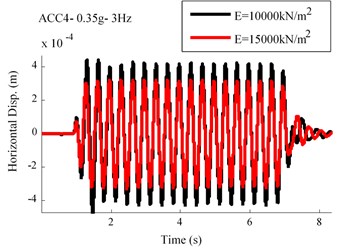
Fig. 15Displacement time history for different values of mass density

5. Conclusions

This study presented an experimental work conducted on a rectangular model tunnel section of Tabriz subway embedded in sand using 1g shaking table. The main focus was to compare the effects of dynamic motions and tunnel flexibility on the tunnel and soil model response. It is observed that:

1) The shear box model with sand has shear wave velocity of approximately 43 m/s which confirms a resonant frequency of 12-16 Hz that has been found from irregular input motions.

2) Accelerations from the soil base towards its surface are amplified within the shear box for all models. Yet, different acceleration discrepancies were observed between FT/RT and FF models. Given the tunnel’s linear behavior, the increase in the magnitude of accelerations from the tunnel base to its roof was higher compared to the free field counterparts.

3) The tunnel and soil responses increase with higher input frequencies.

4) Dynamic bending moments at top corners of the tunnel were found to be larger than those at the bottom corners.

5) Both tunnels behave as a flexible structure with respect to the surrounding soil.

6) A good agreement between the numerical and experimental approaches are obtained.

7) Adopting different values for soil parameters resulted in reasonable soil behaviour in the SBFE-FE model.

References

Hashash Y., Hook J., et al. Seismic design and analysis of underground structures. Tunneling and Underground Space Technology, Vol. 16, Issue 4, 2001, p. 247-293.

Publisher
Hashash Y. M. A., Park D., Yao J. I. C. Ovaling deformations of circular tunnels under seismic loading, an update on seismic design and analysis of underground structures. Tunneling and Underground Space Technology, Vol. 20, Issue 5, 2005, p. 435-441.

Publisher
Huo H., Bobet A., Fernández, Ramírez J. Load transfer mechanisms between underground structure and surrounding ground: evaluation of the failure of the Daikai station. Journal of Geotechnical and Geoenvironmental Engineering, Vol. 131, Issue 12, 2005, p. 1522-1533.

Publisher
Anastasopoulos I., Gerolymos N., Drosos V., Kourkoulis R., Georgarakos T., Gazetas G. Nonlinear response of deep immersed tunnel to strong seismic shaking. Journal of Geotechnical and Geoenvironmental Engineering, Vol. 133, Issue 9, 2007, p. 1067-1090.

Publisher
Anastasopoulos I., Gerolymos, N., Drosos, V., Georgarakos, T., Kourkoulis, R., Gazetas, G. Behavior of deep immersed tunnel under combined normal fault rupture deformation and subsequent seismic shaking. Bulletin of Earthquake Engineering, Vol. 6, Issue 2, 2008, p. 213-239.

Publisher
Amorosi A., Boldini D. Numerical modeling of the transverse dynamic behavior of circular tunnels in clayey soils. Soil Dynamics and Earthquake Engineering, Vol. 59, Issue 6, 2009, p. 1059-1072.

Publisher
Kontoe S., Zdravkovic L., Potts D., Mentiki C. On the relative merits of simple and advanced constitutive models in dynamic analysis of tunnels. Geotechnique, Vol. 61, Issue 10, 2011, p. 815-829.

Publisher
Kontoe S., Avgerinos V., Potts D. M. Numerical validation of analytical solutions and their use for equivalent-linear seismic analysis of circular tunnels. Soil Dynamics and Earthquake Engineering, Vol. 66, 2014, p. 206-219.

Publisher
Baziar M. H., Moghadam M. R., Kim D.-S., Choo Y. W. Effect of underground tunnel on the ground surface acceleration. Tunneling and Underground Space Technology, Vol. 44, 2014, p. 10-22.

Publisher
Bilotta E., Lanzano G., Madabhushi S. P. G., Silvestri F. A numerical Round Robin on tunnels under seismic actions. Acta Geotechnica, Vol. 9, Issue 4, 2014, p. 563-579.

Publisher
Lanzano G., Bilotta E., Russo G., Silvestri F. Experimental and numerical study on circular tunnels under seismic loading. European Journal of Environmental and Civil Engineering, Vol. 19, Issue 5, 2015, p. 539-563.

Publisher
Pitilakis K., Kirtas E., Sextos A., Bolton M., Madabhushi G., Brennan A. Validation by centrifuge testing of numerical simulations for soil-foundation-structure systems. Proceedings of the13th World Conference on Earthquake Engineering, Vancouver, Canada, 2004.

Search CrossRef
Guoxing C., Su C., Xi Z., Xiuli D., Chengzhi Q., Zhihua W. Shaking-table tests and numerical simulations on a subway structure in soft soil. Soil Dynamics and Earthquake Engineering, Vol. 76, 2015, p. 13-28.

Publisher
Penzien J. Seismically induced racking of tunnel linings. Earthquake Engineering and Structural Dynamics, Vol. 29, 2000, p. 683-691.

Publisher
Cilingir U., Madabhushi S. P. G. A model study on the effects of input motion on the seismic behavior of tunnels Soil Dynamics and Earthquake Engineering, Vol. 31, 2011, p. 452-462.

Publisher
Rabeti Moghadam M., Baziar M. H. Seismic ground motion amplification pattern induced by a subway tunnel: Shaking table testing and numerical simulation. Soil Dynamics and Earthquake Engineering, Vol. 83, 2016, p. 81-97.

Publisher
Tsinidis G., Rovithis E., Pitilakis K., Chazelas J. L. Seismic response of box-type tunnels in soft soil: Experimental and numerical investigation. Tunnelling and Underground Space Technology, Vol. 59, 2016, p. 199-214.

Publisher
Deeks A. J., Wolf J. P. A virtual work derivation of the scaled boundary finite-element method for elastostatics. Computational Mechanics, Vol. 28, 2002, p. 489-504.

Publisher
Junyi Y., Feng J., Yanjie X. A seismic free field input model for FE-SBFE coupling in time domain. Earthquake Engineering and Engineering Vibration, Vol. 2, Issue 1, 2003, p. 51-58.

Publisher
Genes M. C., Kocak S. Seismic analyses of soil structure interaction system by coupling the finite element and the scaled boundary finite element methods. International Symposium on Structural and Earthquake Engineering, 2002.

Search CrossRef
Celebi E., Goktepe F., Karahan N. Non-linear finite element analysis for prediction of seismic response of buildings considering soil-structure interaction. Natural Hazards and Earth System Sciences, Vol. 12, 2012, p. 3495-3505.

Publisher
Seiphoori A., Haeri M., Karimi M. Three dimensional nonlinear seismic analysis of concrete faced rock fill dams subjected to scattered P, SV, and SH waves considering the dam-foundation interaction effects. Soil Dynamics and Earthquake Engineering, Vol. 31, 2011, p. 792-804.

Publisher
Bazyar M. H., Basirat B. Dynamic soil-structure interaction analysis under seismic loads using the scaled boundary finite-element method. Journal of Seismology and Earthquake Engineering. Vol. 14, Issue 1, 2012, p. 57-68.

Search CrossRef
Tohidvand H. R., Hajialilue M. Seismic soil structure interaction analysis using an effective scaled boundary spectral element approach. Asian Journal of Civil Engineering, Vol. 15, 2014, p. 501-516.

Search CrossRef
Iai S. Similitude for shaking table tests on soil-structure-fluid model in 1 g gravitational field. Soils Found, Vol. 29, Issue 1, 1989, p. 105-118.

Publisher
Wang J. N. Seismic Design of Tunnels: A Simple State of the Art Design Approach. Parsons Brinckerhoff Inc., New York, 1993.

Search CrossRef

Cited by

A state-of-the-art review on 1-g experimental investigations on tunnels subjected to dynamic loading conditions

Amith K S | Ganesh Kumar S

(2024)

Experimental investigations on the influence of embedment depth and frequency on the dynamic behaviour of tunnels under repeated shaking events

K. Amith | Ganesh Kumar

(2023)

A Numerical Study on Parameters Affecting Seismic Behavior of Cut and Cover Tunnel

Aliakbar Golshani | Mohammadamir Rezaeibadashiani

(2020)

Seismic deformation mode transformation of rectangular underground structure caused by component failure

(2020)

Analytical study of ground responses induced by the excavation of quasirectangular tunnels at shallow depths

Guangshang Zeng | Huaning Wang | Mingjing Jiang

(2019)

Structural components functionalities and failure mechanism of rectangular underground structures during earthquakes

Chao Ma | De-Chun Lu | Xiu-Li Du | Cheng-Zhi Qi | Xiang-Yang Zhang

(2019)

About this article

Received

24 October 2017

Accepted

25 January 2018

Published

30 June 2018

SUBJECTS

Seismic engineering and applications

DOI

https://doi.org/10.21595/jve.2018.19308

Keywords

rectangular tunnel

Tabriz subway

shaking table

physical modeling

scaled boundary finite element method

This is an open access article distributed under the Creative Commons Attribution License, which permits unrestricted use, distribution, and reproduction in any medium, provided the original work is properly cited.

Previous article in issue Previous Next article in issue Next

Research article

2023 05 18

Shaking table test on the dynamic responses of shield tunnel in liquefiable stratum

Yi Feng

Research article

2023 02 17

Shaking table tests of large cross-sectional multi-crack tunnel linings

Dongmei You, Feng Gao

Research article

2022 05 16

Simulation analysis of seismic dynamic response of small interval tunnel in deep backfill area based on model test

Yunchuan Xue, Guodong Sun, Xiaoguang Jin

Research article

2021 01 08

Research on seismic response of new lining structured of shallow double-arch tunnels under unsymmetrical pressure

Hui Yang, Wang Zhou, Xueliang Jiang, Fan Wenchen, Lei Yu

M. Hassanzadeh, M. Hajialilue Bonab, and A. A. Javadi, “Experimental and numerical study of the behavior of shallow rectangular tunnels,” Journal of Vibroengineering, Vol. 20, No. 4, pp. 1783–1796, Jun. 2018, https://doi.org/10.21595/jve.2018.19308

Copy Extrica

Copied to clipboard!

TY  - JOUR
DO  - 10.21595/jve.2018.19308
UR  - https://doi.org/10.21595/jve.2018.19308
TI  - Experimental and numerical study of the behavior of shallow rectangular tunnels
T2  - Journal of Vibroengineering
AU  - Hassanzadeh, Mehran
AU  - Hajialilue Bonab, Masoud
AU  - Javadi, Akbar A.
PY  - 2018
DA  - 2018/06/30
PB  - JVE International Ltd.
SP  - 1783-1796
IS  - 4
VL  - 20
SN  - 1392-8716
SN  - 2538-8460
ER  - 

Copy Ris

Copied to clipboard!

@article{Hassanzadeh_2018,
	doi = {10.21595/jve.2018.19308},
	url = {https://doi.org/10.21595/jve.2018.19308},
	year = 2018,
	month = {jun},
	publisher = {{JVE} International Ltd.},
	volume = {20},
	number = {4},
	pages = {1783--1796},
	author = {Mehran Hassanzadeh and Masoud Hajialilue Bonab and Akbar A. Javadi},
	title = {Experimental and numerical study of the behavior of shallow rectangular tunnels},
	journal = {Journal of Vibroengineering}
}

Copy Bibtex

Copied to clipboard!

[1]M. Hassanzadeh, M. Hajialilue Bonab, and A. A. Javadi, “Experimental and numerical study of the behavior of shallow rectangular tunnels,” Journal of Vibroengineering, vol. 20, no. 4, pp. 1783–1796, Jun. 2018, doi: 10.21595/jve.2018.19308.

Copy IEEE

Copied to clipboard!

Hassanzadeh, Mehran, Masoud Hajialilue Bonab, and Akbar A. Javadi. “Experimental and Numerical Study of the Behavior of Shallow Rectangular Tunnels.” Journal of Vibroengineering 20, no. 4 (June 30, 2018): 1783–96. https://doi.org/10.21595/jve.2018.19308.

Copy Chicago

Copied to clipboard!

Experimental and numerical study of the behavior of shallow rectangular tunnels

Abstract

1. Introduction

2. Shaking table testing

2.1. Shaking table facility of University of Tabriz

2.2. Soil and model tunnels

2.3. Model preparation and instrumentation

2.4. Loading characteristics

3. A brief description of the scaled boundary finite element method

4. Results and discussion

4.1. Hammer test

4.2. Soil and tunnel horizontal acceleration

4.3. Bending moment of tunnel lining

4.4. Soil-tunnel flexibility ratios

4.5. Numerical parametric study

5. Conclusions

References

Cited by

About this article

Related Articles