Optimizing SVM’s parameters based on backtracking search optimization algorithm for gear fault diagnosis

1. Introduction

The gearbox is the most crucial transmission mechanism in a rotating machine, and the implementation of online monitoring and diagnosis has become quite urgent and necessary. The vibration signal of a gearbox contains much noise and unstable factors thus the vibration signal is a typical non-stationary signal. The fault signal characteristic is very weak and is usually masked by noise, especially when the fault is in its early stages; thus, it is very difficult for getting the fault features [1]. There are three steps in diagnosing fault gears, namely: characteristic signal detection, feature extraction and fault classification. Generally, the process of extracting the features of faults is divided into selection and extraction. In both theoretical and experimental fields, the fact of selection and extraction of fault features is the common principle in diagnosing faults. Feature extraction is an important step in the fault identification. In case of incorrect or incomplete feature extraction, it unavoidably leads to the fact that the classification and false diagnosis are made with errors [2]. So, the extraction of the effective information about the fault characteristics from complex dynamic mechanical signals is the key factor to solve the problem of large-scale complex mechanical and electrical equipment fault diagnosis.

The corresponding characteristics of the vibration signals will be presented, and getting the extraction of the fault information of a non-stationary vibration signal is the crux of gear fault diagnosis. Vibration signals are usually processed by decomposing the original signal, such as fast Fourier transform, wavelet transform, Hilbert-Huang transform and EMD method [3]. This is one of the efficient techniques in diagnosing faults based on of time-frequency resolution, i.e. EMD is rather good at extracting the Intrinsic Mode Functions (IMFs), or mono-component functions embracing the original signal [4]. But the EMD method has several shortcomings, such as the problem of mode mixing, distorted components and time-consuming decomposition [5]. To this end, Wu and Huang have proposed a method namely EEMD [6]. Pattern recognition is another side in diagnosing gear faults.

Recently, Cheng et al. have developed a new novel signal decomposition approach named as the local characteristic scale decomposition (LCD). Similar to the EMD, the LCD method is used to decompose a complex signal into several ISCs and a residue [7]. Because the LCD is the same EMD method, it is a kind of data-driven and adaptive non-stationary signal decomposition, so it is suitable for processing non-stationary signals such as vibration signals of gears.

Support vector machine (SVM) proposed by Vapnik et al. is a promising classification method and has been successfully applied to many engineering fields, such as face recognition, credit scoring and mechanical fault diagnosis, etc. [8]. SVM has the high generalization ability that depends on the adequate setting of parameters such as penalty coefficient $C$ and kernel parameters $\sigma$. Therefore, the selection optimal parameters are essential and important to obtain a good performance in handling learning task of SVM [9]. In the past several years, the optimal SVM has gained great attentions. There are several methods for setting the parameters of SVM such as the grid search, the cross-validation method, and the gradient descent method [10]. These methods have several drawbacks; for example, the performance of grid search is sensitive to the setting of the grid range and coarseness for each parameter, which is not easy to be set without prior knowledge, and the cross-validation method requires long and complicated calculations.

The Backtracking Search Algorithm (BSA), which has been developed by Civicioglu, is an evolutionary algorithm (EA) to solve problems of real-valued numerical optimization. Selection, mutation and crossover are three well-known operators which are based on the BSA method but others like the genetic algorithm (GA) and differential evolution (DE) [11]. Furthermore, unlike many other metaheuristics, the BSA algorithm has only one control parameter and is not very sensitive to the initial value as reported therein. Since it had been introduced, the BSA attracted many researches, and it was applied to various optimization problems. Some successful examples are described below. In [12], a comparative analysis of BSA with other evolutionary algorithms for global continuous optimization was given. In [13], the BSA was used for the antenna array design. In [14], the BSA was employed for the design of robust Power System Stabilizers (PSSs) in multi machine power systems. In [15], it was used for the allocation of multi-type distributed generators along distribution networks [16]. The problems of real-valued numerical optimization were quickly resolved by the BSA method, and the experiments demonstrated better results than EAs. Because of applying only one control parameter, thereby, researchers got more advantages in conducting experiments. For analyzed positive point, the paper will apply BSA in the combination with the SVM aiming at diagnosing faults gears, so-called BSA-SVM.

In this paper, the MPE-LCD based on BSA-SVM is used to diagnose and classify gear faults. Firstly, the original vibration signal is decomposed by the LCD method into some ISC components. Then, the first few ISCs are chosen and extracted the fault feature vectors by the MPE algorithm [17]. Thirdly, in order to identify the work condition of gear, in this paper, the SVM is served as a classifier [18]. Furthermore, the authors proposed a new optimal algorithm named as BSA to make the optimization for the SVM parameters (BSA-SVM). The characteristic vectors of the stationary ISCs are taken as the input data of the BSA-SVM, and then the gear faults and the normal gear condition can be differentiated [7]. Furthermore, to ascertain the superiority of the MPE-LCD based on BSA-SVM, it is compared with EMD and EEMD combined with GA-SVM, PSO-SVM and SVM. The analysis results show that the diagnosis approach of BSA-SVM assisted with MPE-LCD is suitable for processing non-stationary signals, such as vibration signals of gears, with a higher accuracy and effect when compared to other methods.

The content of the paper composes as: Section 2 and 3 are dedicated to the LCD and MPE methods. In Section 4, the parameter optimization algorithm based on the BSA method is addressed. Section 5 refers to characteristic energy extracted from a number of ISCs which played as input vectors of BSA-SVM. The most important content will be shown in Section 6. This not only introduces the optimization algorithm linked to BSOA-SVM and LCD but indicates its strong points in practice. Eventually, Section 7 will make some conclusions.

2. Local characteristics-scale decomposition method

Similar to EMD, the LCD is a self-adaptive data decomposition method. Based on the local characteristic scale, the LCD establishes a new definition of a mono-component with physical meaning [19]. Any complex signal $x\left(t\right)$ can be decomposed into several ISCs and the residue by using the LCD [18], as follows:

where $c_i\left(t\right)$ is the $i$th ISC and $r_n\left(t\right)$ is the residue. The assessment criterion for ISC is as follows: all the maxima are positively, and all the minima are negatively in the whole data set. As shown in Fig. 1, any two adjacent maxima (minima), ($t_{k-1}$, $x_{k-1}$) and $(t_{k+1},x_{k+1})$ are connected by a straight line. To the intermediate minima (maxima) ($t_k$, $x_k$), its corresponding point ($t_k$, $A_k$) on this straight line is as follows:

For assuring the smooth and symmetric features of the ISC, the proportions of $x_k$ and $A_k$ remain constant, as follows:

where $a$ is a proportional coefficient. When $a$ is a constant, the proportions of $x_k$ and $A_k$ can remain constant. Generally, $a$ is set as 0.5, thus, $A_k/x_k=$ –1. At this time, $x_k$ and $A_k$ are symmetrical for the $x$-axis ensuring the symmetric feature of the achieved ISC.

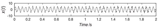
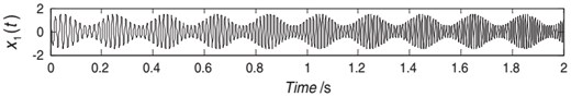
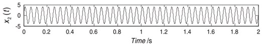
Without losing the generality, the signal is shown as:

where:

In Fig. 1 the waveforms of $x\left(t\right)$, $x_1\left(t\right)$ and $x_2\left(t\right)$ are shown.

As a constant sequence or monotonic sequence, $r_n\left(t\right)$ represents the average trend of the signal generally. The ISC component $c_i\left(i=1,\dots ,n\right)$ represents a signal of different frequencies from high to low. The signal frequency component in each frequency band changes according to the original signal. The decomposition process of the LCD is as follows (the whole decomposition process ends when the SD criterion [17] is satisfied, and a value of SD = 0:3 was set in this study):

(1) Assume the number of extrema of the signal $x\left(t\right)$ is $M$, and determine all the extrema ($t_k$, $x_k$) ($k=1,\dots ,M$) of the signal $x\left(t\right)$.

(2) Compute $A_k$($k=1,\dots ,M$) according to Eq. (2), and calculate the corresponding $L_k$ ($k=1,\dots ,M$) according to Eq. (3):

where $a=$ 0.5. When calculating $A_1$, ($t_0$, $x_0$) needs to be extended by the image method [18]. Similarly, $A_M$ can be calculated after ($t_{M+1}$, $x_{M+1}$) is extended [20].

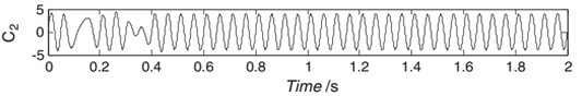
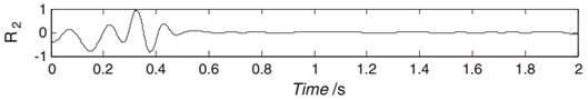
Fig. 1Waveform of signal: a) xt, b) x1t, c) x2t

a)

b)

c)

Fig. 2Result of signal (10) decomposed by EMD

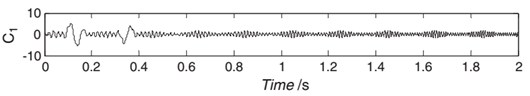
a)

b)

c)

Fig. 3Result of signal decomposed by LCD

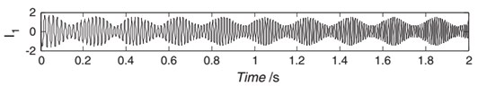
a)

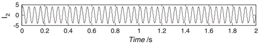
b)

c)

(3) All the $L_k\left(k=1,\dots ,M\right)$ are connected by a spline line $S{L}_1\left(t\right)$, which is defined as the base line of the LCD. By contrast, EMD's base line is defined as the mean of the upper and the lower envelopes.

(4) The difference between the data and the base line $S{L}_1\left(t\right)$ is the first component $h_1\left(t\right)$:

If $h_1\left(t\right)$ is an ISC, take it as the first ISC of $x\left(t\right)$. Otherwise, take it as the original signal and repeat the above process until $h_m\left(t\right)$ is an ISC after $m$ iterations of the computation. Afterwards, $h_m\left(t\right)$ is expressed as the $IS{C}_1$.

(5) Separate the first $IS{C}_1$ from $x\left(t\right)$:

(6) Take the residue $r_1$ as the original signal to be processed. Repeat the above process until $IS{C}_1,\dots ,IS{C}_n$ and the residues are obtained, as shown in Eq. (1).

The original signal is disintegrated into several ISCs by applying LCD, and the first few ISCs have the highest frequency and largest energy, while the last few ISCs remain relatively moderate. However, high frequency modulations still exist, which can interfere with the feature extraction. The TEO is used to demodulate the obtained ISC signal in this paper.

3. Permutation entropy (PE) and multi-scale permutation entropy (MPE)

4. BSA and parameter optimization of SVM based on BSA

4.1. Backtracking search optimization algorithm

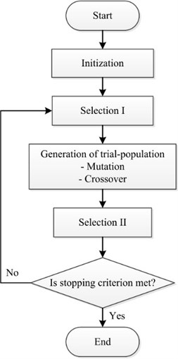
The main content of BSA method is to generate a trial population including two new crossover and mutation operators. The BSA strategy is considered as powerful exploration because this method both generates trial populations and controls the amplitude of the search-direction matrix and search-space boundaries [21]. Particularly, the BSA stores a population from a randomly chosen previous generation to use it in generating the search-direction matrix. The BSA strategy is very strong in terms of both a global exploration and local exploitation with a good feature of local minima avoidance [22, 23]. The main five procedures of the BSA method are presented as follows in Fig. 5.

Problem and Algorithm Parameter: An overview of five processes is provided as follows.

Fig. 4Flow chart of backtracking search optimization algorithm

4.1.1. Initialization

The procedures of BSA begin from initializing the population $P$ as follows:

15

$P_{i,j}={lower}_j+\left({upper}_j-{lower}_j\right)\times random,i=\mathrm{1,2},\dots ,NP,j=\left(\mathrm{1,2},\dots ,DP\right).$

In which: NP is the size of population (Pop Size). DP is the dimensional number of the problem. random is a real value which is uniformly allocated between 0 and 1. $lowe{r}_j$ stands for the lower bound for the $j$th factor of the $i$th individual. $uppe{r}_j$ is the upper bound for the $j$th factor of the $i$th individual.

4.1.2. Selection-I

The generation of $oldP$ is the historical population, in the procedure of the Selection-I, and it is used to make a calculation for the search direction. The formulation is as follows:

16

$P_{i,j}={lower}_j+\left({upper}_j-{lower}_j\right)\times random,i=\mathrm{1,2},\dots ,NP,j=\left(\mathrm{1,2},\dots ,DP\right).$

In each iteration, $oldP$ is defined as follows:

17

$\text{if}\mathrm{}\mathrm{}a<b\text{then}oldP≔P\left|a,b\right.\in \left[\mathrm{0,1}\right].$

In which: $≔$ means the updated operation. Two random numbers, $a$ and $b$, are within the range [0, 1]. The above equation assures that the BSA algorithm population might be randomly chosen from a historical population. The algorithm memorizes the historical population till it is changed via a random permutation.

4.1.3. Mutation

Initially, the trial population is created via mutation operation as per the bellow formulation:

18

$T=P+\left(oldP-P\right)\times F,$

where $F$ is a scale factor which controls the amplitude of mutation ($oldP-P$).

In this paper, $F=3•random$, where $random$ is a random real number with uniform distribution within the range (0, 1). By involving the historical population in calculating $oldP-P$, BSA learns from its memory of previous generations to obtain a trial population [24].

4.1.4. Crossover

The final trial population $T$ is generated by crossover. The guidance of the trial individuals characterized by improved fitness values supports the search direction in optimizing the problem. BSA crossover works as the following procedure. A binary integer-valued matrix (map) of size $NP\times DP$ is computed in the first step.

The individuals of $T$ are generated by utilizing relevant individuals of $P$. If ${map}_{i,j}=$ 1, $T$ is updated with $T_{i,j}:=P_{i,j}{P}_{i,j}$.

4.1.5. Selection-II

In the stage of Selection-II, $T_i$ makes the corresponding $P_i$ better in the manner of fitness value which is utilized for updating $P_i$ [21]. As the BSA finds the best optimal value ($P_{best}$) which is dominant comparing to all previous ones, $P_{best}$ takes the place of all optimal solutions, and these values are updated as the most fitting value of $P_{best}$.

4.2. SVM parameter optimization based on BSA

4.2.1. Support vector machine (SVM)

The SVM is a type of machine learning technique. The SVM relies on the theory of statistical learning. The SVM is handling the training samples as the input to a higher-dimensional characteristic space through the use of a mapping function ${\varphi }^7$. Assuming that there is a given set of the training samples $G=\left\{\left(x_i,y_i\right),i=\mathrm{1,2},...,l\right\}$in which each sample $x_i\in R^d$belongs to a class by $y\in \left\{+1,-1\right\}$, and the training data is not linearly separable in the space of feature, then the target function can be expressed as follows [17]:

19

$\mathrm{M}\mathrm{i}\mathrm{n}\mathrm{i}\mathrm{m}\mathrm{i}\mathrm{z}\mathrm{e}\varphi \left(\omega \right)=\frac{1}{2}⟨\omega .\omega ⟩+C{\sum }_{i=1}^l{\xi }_i,y_i\left(⟨\omega .\varphi \left(x_i\right)⟩+b\right)\ge 1-{\xi }_i,$
${\xi }_i\ge 0,i=\left\{\mathrm{1,2},\dots ,l\right\}.$

In which $\omega$ is the normal vector of the hyperplane, $C$ is the penalty parameter, $b$ is the bias, ${\xi }_i$is non-negative slack variables, and $\varphi \left(x\right)$ is the mapping function.

By introducing a set of Lagrange multipliers ${\alpha }_i\ge$ 0, the optimization problem could be rewritten as:

20

$\text{Maximize}\mathrm{}L\left(\omega ,b,\alpha \right)={\sum }_{i=1}^l{\alpha }_i-\frac{1}{2}{\sum }_{i,j=1}^l{\alpha }_i{\alpha }_j{y}_i{y}_{j}K\left(x_i{x}_j\right),$
$0\le {\alpha }_i\le C,{\sum }_{i=1}^l{\alpha }_i{y}_i=0.$

The function of making decision can be achieved as:

21

$f\left(x\right)=\mathrm{s}\mathrm{g}\mathrm{n}\left[{\sum }_{i=1}^l{\alpha }_i{y}_{i}K\left(x_{i}x\right)+b\right].$

The SVM method used the radial basis kernel function which is the most common kernel function as it indicates in the bellow equation:

22

$K\left(x{x}_i\right)=\mathrm{e}\mathrm{x}\mathrm{p}\left(-\frac{{‖x-x_i‖}^2}{2{\sigma }^2}\right),$

where $\sigma$ is the kernel parameter.

4.2.2. SVM’s parameter optimization relied on BSA

The performance of SVM is significantly impacted by its parameters. It needs to be selected as a penalty factor $C$ and kernel parameter $\sigma$ in the function of Gaussian kernel. It is not easy to select these parameters. As a whole, $C$ and $\sigma$ are chosen empirically. Therefore, this paper applied the BSA as a technique for optimizing the parameters of SVM. As a consequence, $C$ and $\sigma$ played as the variables. SVM error testing became the fitness function for the sake of optimization.

The SVM error testing is made as:

23

$\text{fitness}\left(x\right)={Tes{t}_{Error}}_{SVM}\left(x\right),$

where $x=\left(C;\sigma \right)$ and the test error of SVM was defined as:

24

${Tes{t}_{Error}}_{SVM}=\left(1-\frac{y_f}{y_t+y_f}\right)100\%,$

where $y_t$ and $y_f$ mean the numbers of true and false classified samples, respectively. The desirable value is too small to ensure high classification accuracy.

4.2.3. Experimental results

The paper used Thyroid, Seed and Escherichia coli (E. Coli) as three common sets of benchmark data provided by the University of California, Irvine to quantify the performance of the suggested BSA-SVM method.

Table 1 showed the training and test sets. Every sampling set is separated into two subsets. In which, one subset is used for SVM training, and the other is for testing the obtained model. The training set accounted for 70 %, and the test set took 30 % of the total samples. Based on the trial and error detection practice, this proportion was selected in order to evaluate the performance of the achieved SVM which was optimal for the available samples.

Three data sets were used to make classification among the BSA-SVM, GA-SVM, PSO-SVM, and CMAES-SVM methods. The values selection is the same in all four above methods in order to make comparison fairly (e.g., iteration = 30 and Pop Size = 30). For the PSO, the parameters were fixed with the values given in the literature [22, 26] (i.e., $W=$ 0:9, $c_1=$ 0:5, and $c_2=$ 1:25). For CMAES, the parameters were fixed with the values given in the literature [24] (i.e., ${\sigma }_0=$ 0:25 and $\mu =4+3\mathrm{l}\mathrm{o}\mathrm{g}\left(N\right)$). Each testing method result was considered as the average value of 30 runs. The training data and test data were both mixed and were randomly divided, as shown in Table 1.

Lin et al. argued that [25] the lower and upper bounds of $C$ were given in [0:01; 35000] and $\sigma$ in [0:01; 32] for the BSA-SVM, GA-SVM, PSO-SVM, and CMAES-SVM classifiers. Each search method gave the values of $C$ and $\sigma$ in order to give the smallest value of the classification error. Table 2 presented experimental results.

The effectiveness of the proposed method was illustrated in Tables from 2 to 4 on the basis of the detailed classification results of each data set. The Thyroid and Seed data sets encompassed three classes, thus, the authors needed two SVM classifiers. The E. Coli data set embraced five classes; therefore, the authors needed four classifiers. These tables show the optimal parameters ($C$ and $\sigma$), average test error, and average cost time done by different algorithms.

Fig. 5Parameter optimization flowchart of SVM based on BSA

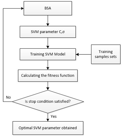
Table 1Parameters of datasets

Name	Data	Train	Test	Validation data	Input	Class
Thyroid	215	151	52	150	5	3
Seed	210	147	55	160	7	3
E. coli	327	229	60	180	7	5

Table 2Results of thyroid data set

Method	Training samples	Test samples	Average cost time (s)	Average test errors (%)	Refs.
BSA-SVM	150	52	15.83	0.000	[25]
PSO-SVM	150	52	36.31	2.358	[26]
GA-SVM	150	52	31.12	1.442	[27]
CMAES-SVM	150	52	32.56	2.622	[28]

Table 3Results of seed data set

Method	Training samples	Test samples	Average cost time (s)	Average test errors (%)	Refs.
BSA-SVM	160	55	17.65	0.910	[25]
PSO-SVM	160	55	40.69	3.993	[26]
GA-SVM	160	55	36.38	3.552	[27]
CMAES-SVM	160	55	37.56	2.298	[28]

The results of the E. Coli, Seed and Thyroid classification were given in Table 1. The next Table indicates that the cost timing and testing error of BSA-SVM was a bit lower in comparison with those of other methods as GA-SVM, PSO-SVM, and CMAES-SVM. Civicioglu said that the BSA utilized a mutation mechanism in which there was a complex crossover and one individual [25]. Moreover, by using its memory, the BSA took an advantage of the experiences achieved from previous generations. Tables 2-4 demonstrate that the BSA-SVM classifier achieved higher classification accuracy in the way of a shorter time as comparing to other methods. Next, the BSA-SVM method was used to diagnose a gear fault.

Table 4Results of E. Coli data set

Method	Training samples	Test samples	Average cost time (s)	Average test errors (%)	Refs.
BSA-SVM	180	60	26.73	4.641	[25]
PSO-SVM	180	60	59.43	5.364	[26]
GA-SVM	180	60	44.78	7.787	[27]
CMAES-SVM	180	60	42.52	8.582	[28]

5. Gear fault diagnosis method based on BSA-SVM and LCD-MPE

Sections 2 and 3 showed the applied LCD in the combination with the MPE under different work status to analyze a gear vibration signal. Thereby, fault patterns are clearly recognized via the energy of each ISC changed when the gear malfunctioned. The BSA-SVM input vector is the energy feature of every ISC component. By doing so, the work status and fault patterns of the gear can be identified.

Fig. 6Flowchart chart of gear fault diagnosis based on LCD-MPE and BSA-SVM

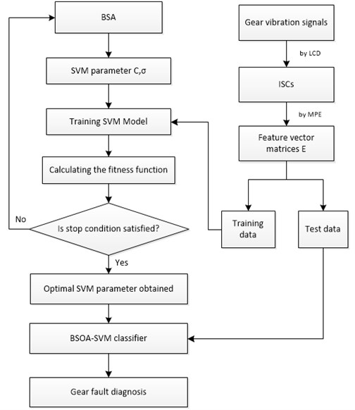
Fig. 6 shows the flow chart of the LCD-MPE and BSA-SVM method for the gear fault diagnosis. The description of the method for diagnosing gear faults is as follows:

(1) Choose several signals as samples under three cases: gear normal, gear chipped, and gear broken.

(2) Disintegrate the original vibration signals by the LCD method into several ISCs. The first mISCs which include the most dominantly information of the fault gear will be chosen to extract the feature.

(3) Calculate MPE for each gear vibration signal getting from the first $m$ ISCs with the parameter selection: $m=$ 6; $\tau =$ 1; $N=$ 2048, and the maximum scale factor $t_{max}=$ 12.

(4) Then the MPEs are obtained in all scales, and are viewed as the feature vector $E$ to represent the main fault information of gear vibration signal.

(5) Run the BSA-SVM, with the parameters of SVM, named as $N$ and $\sigma$, which are optimized by the BSA.

(6) Input the vector $E$ into the BSA-SVM classifier and realize training. The fitness function is given by Eq. (21). The net results of $N$ and are input to the BSA-SVM classifier.

(7) The output of BSA-SVM is defined with the work conditions of the gear with three classes: class 1 – normal [–1 –1 +1]; class 2 – chipped tooth [–1 +1 –1]; class 3 – broken tooth [+1 –1 –1].

6. Application of BSA-SVM and LCD-MPE to diagnose gear faults

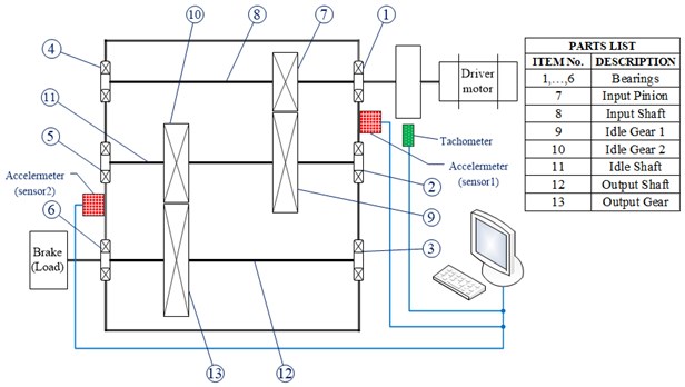
Data collected in this paper comes from the public data sets distributed by the Prognostics and Health Management (PHM) Society [29], and the data sets were sampled synchronously from two accelerometers mounted on each side of the gearbox housing shown in Fig. 7. Data collection was implemented at five different shaft speeds of 30, 35, 40, 45 and 50 Hz under a low and high load from the brake with the sample frequency $fs=$ 200/3 kHz. The low and high loads have resulted in a small difference of shaft speed, each load case is repeated four times. There are totally 560 different cases to be diagnosed, with six cases using helical gears and the other eight spur gears. On the input shaft, the tachometer generates 10 pulses per revolution and data from the tachometer is very accurate. Here we chose the helical gear to research with three states: normal, chipped tooth and broken tooth, and the sampling frequency can be taken as 1024 Hz. The vibration signals of helical gear with three conditions (normal, chipped tooth and broken tooth) were tested, and 40 vibration signals from the helical gear in each condition were taken from 6 groups collected at random as the test data.

Fig. 7Common test rig

Firstly, the vibration signals of each group with three conditions named as normal, chipped tooth and broken tooth were decomposed by LCD-MPE into a number of ISCs. The first seven ISCs embrace the most dominant information which is selected and arranged in accordance with the frequency components as $c_1\left(t\right),c_2\left(t\right),\dots ,c_8\left(t\right)$ from high to low. Then, the fault features vector $T$ was obtained following the MPE method. Finally, the BSA-SVM was used to identify the various patterns. In order to have a fair comparison, the original vibration signals are chosen similarly. These signals are decomposed by LCD into ISCs, of which, the first eight IMFs are selected and arranged in the manner of high to low values basing on frequency components as $c_1\left(t\right),c_2\left(t\right),\dots ,c_8\left(t\right)$. And then, the feature vector is taken into the input of BSA-SVM. The identification results for the test samples based on LCD-MPE and compared with EMD and EEMD method are shown in Table 5.

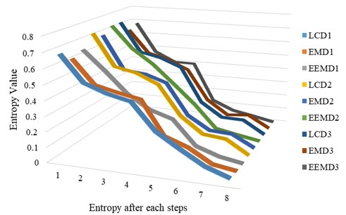
The input vector of the BSA-SVM method uses the LCD or EMD analysis as preprocessor to extract the energy in each frequency band in identifying the fault gears. These input vectors affect the identification of the fault gears. The frequency components after decomposition by LCD-MPE has better results than the ones in the EMD and EEMD method, therefore, the method BSA-SVM based on LCD is better than that based on EMD. The experimental results were demonstrated in Table 5 and Fig. 8. As a result, the accuracy of identification is good, and the time is shorter. In practical cases, they may be used for a fault diagnosis.

Fig. 8Results based on LCD-MPE or EEMD for gear fault diagnosis

7. Conclusions

Basing on the feature of non-stationary of gear fault signals, a method of diagnosing a faulty gear based on the LCD-MPE and BSA-SVM is proposed. LCD and MPE were firstly used to pre-process different types of vibration signals. BSA was then employed to make the optimization for the parameters of SVM aiming at increasing the sensitivity and accuracy of SVM. This combination used to classify data of the work condition of the gear is called as BSA-SVM. When the working condition of gear changes, then the fault feature extraction is also changed indicating that the energy of each frequency component is changed when the gear with different faults is operating. Thus, the feature vector of each ISC component is adopted as input features for BSA-SVM to identify the gear work condition. Based on experimental results, some conclusions of the paper are:

(1) LCD is a method of processing self-adaptive signals, which can be applied to nonlinear and non-stationary processes faultlessly.

(2) BSA is an optimal algorithm that is used to make the optimization for the parameters of SVM network. Experimental results above show that the BSA and SVM combine better than other optimization algorithms (GA, PSO) combined with SVM.

(3) The successful combination of LCD-MPE with BSA-SVM identifies the work condition and fault patterns for the gears and provides an effective tool for intelligent fault diagnosis of gears.

(4) The BSA-SVM method that took the fault feature vector of each frequency component based on LCD combined with MPE as the input features has greater identification power than that based on EMD or EEMD combined with MPE.

In short, the paper presents another approach to gear fault diagnosis using a chain of data mining methods. Firstly, the LCD is used for vibration signals decomposition. The LCD is an improved form of the Huang-Hilbert Transform. Thanks to this, the problem of the mode mixing in this transform is removed. It is well visible in diagnosis results presented in Table 5. Next, the MPE is calculated as a feature characterizing each ISC obtained after signal decomposition by the LCD method. Then the MPEs values obtained in all scales are used as the feature vector to SVM classifier. However, the paper authors have improved the effectiveness of this classifier by optimizing its parameters with the aid of backtracking search optimization algorithm (BSA). Thanks to such a novel approach to the whole procedure of data mining applied to gear fault diagnosis they propose a very effective methodology which is able to perform the bearing different fault type diagnosis in a very reliable and robust way. According to the results presented in Table 5, the combination of LCD-MPE with BSOA-SVM can identify the work condition and fault patterns of the gears with the test error equal to 0 % for all the tested cases.