Numerical simulation of hydraulic fracturing in transversely isotropic rock masses based on PFC-2D

In order to make a better understanding of the hydraulic fracturing in transversely isotropic rock masses, the modified particle flow modeling method was used by embedding the smooth joint models within an area of certain thickness, and the optimized fluid-mechanical coupling mechanism was applied in hydraulic fracturing modeling. On this basis, the influence of the injection rates, in-situ stress ratios and inclination angles of the bedding planes on the breakdown pressure and propagation of the hydraulic fractures was analyzed. The simulation indicated that: 1) Excessive small or large injection rates would lead to the increase of the breakdown pressure of the hydraulic fractures. 2) Under different inclination angles of the bedding planes, the crack breakdown pressure increased linearly with the increasing of the in-situ stress ratios. And under conditions of different in-situ stress ratios, the crack breakdown pressure changed as a ‘wave’ type with the increasing inclination angles of bedding planes. 3) Both the in-situ stress ratios and the inclination angle of bedding planes affected the propagation of the hydraulic fractures. The existence of the bedding planes would induce the hydraulic fractures to propagate along the bedding planes. The large inclinations of the bedding planes would cause the hydraulic fractures to keep propagating with the direction of maximum principal stress.

$Numerical simulation of hydraulic fracturing in transversely isotropic rock masses based on PFC-2D$

Highlights

The optimized particle flow modeling method was used to simulate the hydraulic fracturing.
The crack breakdown pressure changed as a wave type with different inclination angels.
Bedding planes would induce the hydraulic fractures to propagate along the bedding planes.

1. Introduction

In recent years, with the success of the shale gas revolution in the United States, the unconventional oil and gas resources have been developed efficiently and economically. This is due to the fact of the rapid development of the horizontal drilling and multi-stage hydraulic fracturing. Through the horizontal drilling and multi-stage hydraulic fracturing, complex fracture networks can be formed in low-porosity and low-permeability rock formations, such as the shale reservoirs. And the volume of reconstruction can be increased to improve the exploitation efficiency of the reservoir. However, due to the complexity of the rock mass and the invisibility of the reservoir, the fracture and propagation process cannot be monitored directly in actual engineering projects. In order to apply the hydraulic fracturing techniques better, the process of the hydraulic fracturing is needed to be studied in detail. Based on these, many researchers have conducted in-depth studies on the fluid-driven fracturing processes, including the interaction between natural fractures and hydraulic fractures. Lichu Jia [1], Yush Zou [2] used the X-ray computer tomography technology to scan the rock samples before and after fracturing to observe the hydraulic fractures and to study the interaction between the hydraulic and natural fractures during the propagation process. Sergey Stanchits et al. [3] used acoustic emission technology to monitor the fracture position during the fracturing process, and obtain the relationship between the hydraulic fractures and the natural fractures under the different injection rate and fluid dynamic viscosity. Shuai Heng et al. [4] conducted a series of true triaxial hydraulic fracturing tests with shale. The influence of the bedding planes on the propagation of hydraulic fractures was studied based on the instability propagation criterion of tensile fractures. Due to the disadvantages of the high cost and complicated operation of experimental tests, more researchers preferred to use numerical simulation method to study the initiation and propagation of the hydraulic fractures in natural fractured rock masses. McClure [5] used two-dimensional displacement discontinuous method (DDM) to study the propagation of hydraulic fractures in rock reservoirs with natural discrete fracture networks. Kresse et al. [6] introduced three-dimensional correction factor to compensate for the effect of fracture height in 2D-DDM, and to establish a complex hydraulic fracture network model (HFN) to study the stress shadow effect. Hanyi Wang [7] established a fully coupled non-planar hydraulic propagation model using the XFEM (Extended Finite Element Method) to study the initiation and propagation of hydraulic fractures in brittle and ductile rock masses. Qingdong Zeng et al. [8] established a multi-crack synchronous propagation mathematical model, and conducted numerical simulations in horizontal wells based on XFEM. Zuorong Chen et al. [9] used the cohesive-zone crack tip model to replace the stress intensity model, simulating the propagation of hydraulic fractures in ABAQUS. Yu Wang et al. [10] applied RFPA-Flow calculation software to analyze the stress shadow in hydraulic fracturing under different analytical factors, such as well spacing, in-situ horizontal stress difference coefficient and rock heterogeneity. Chengzeng Yan [11-13] proposed a theoretical framework for the fluid-mechanical coupling with FDEM (Finite-Discrete element Method). Combined with the recursive search algorithm for the formation of fractured network, it provided a new approach for simulating the hydraulic fracturing problems in low-permeability rock masses.

As one of the most rapidly developing areas of computational mechanics, the discrete element method (DEM) in particulate and blocky systems has undergone a significant development in the past decades. As a discrete element approach, the major advantage of BPM (Bonded-particle Model) is that complex empirical constitutive behavior can be replaced by simple particle contact logic [14]. Moreover, the cracks which are simulated by the DEM are formed by the interpenetrating of many micro-cracks, and the crack propagation has better randomness. Compared with the finite element method, the discrete element models do not need to preset the cells with where the fracture would happen during the loading process. The micro-cracks can be formed spontaneously according to the mutual transfer of force and displacement between particles. Thus, the DEM can simulate the crack initiation, propagation and penetration more realistically. The particle discrete element method, which is a distinct element-based model [15], has been widely used in rock fracture research [14, 16-17] and hydraulic fracturing [18-25]. Since unconventional oil and gas reservoirs, such as shale, have the distinct layered structure, the bedding planes will affect the initiation and propagation of the hydraulic fractures. In this paper, the numerical model of transversely isotropic rock masses was built by embedding smooth joint models (SJM). And based on the mechanism of the fluid-mechanical coupling in PFC, the crack initiation and propagation of hydraulic fractures in transversely isotropic rock masses were studied.

2. Mechanism of fluid-mechanical coupling in PFC

2.1. Basic assumptions

The mechanism of fluid-mechanical coupling is mainly based on the two basic assumptions [26]:

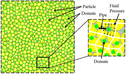
(1) It is assumed that the percolation path was along the parallel plate channels located at the contacts between the particles. This channel is called the ‘pipe’, as shown in Fig. 1 by the black line (The yellow circle in the figure indicates the solid particle and the white line indicate the contact between the particles).

(2) There is a unit in the model that can store fluid pressure, which is called the ‘domain’, as shown in Fig. 1. The closed polygon element surrounded by white segments is the domain and the green circle indicates the center. The adjacent domains are connected by the pipes. The fluid pressure in the domain exerts fluid traction force on the enclosing particles as shown by the arrows in the domains.

Fig. 1PFC model for mechanism of fluid-mechanical coupling

2.2. Calculating theories

(1) Changes of the liquid flow in the domain.

The different liquid pressures contained in the adjacent domains will induce the seepage of the liquid flow in the two domains, and the exchanging channel is the pipe located at the contact between the particles. The seepage discharge q between the adjacent domains is determined by the hydraulic aperture $a$ , the fluid pressure in the adjacent domains ( $P_{1}$ , $P_{2}$ ) and the fluid dynamic viscosity $μ$ . The relationship between them is the Cubic law [28] as shown in Eq. (1):

1

q = \frac{a^{3}}{12 μ} \frac{p_{2} - p_{1}}{L} .

(2) Hydraulic aperture.

It can be seen in Eq. (1) that the change of the liquid flow in the domains is mainly determined by the hydraulic aperture $a$ . In the numerical models, the hydraulic aperture is set as a function related to the contact force between the particles [27]:

2

a = a_{i n f} + (a_{0} - a_{i n f}) e x p (- 0.15 σ_{n}) .

In which the $σ_{n}$ represents the effective normal stress at the contact (units in MPa). When $σ_{n}$ tends to infinity, the hydraulic aperture decreases asymptotically to infinite hydraulic aperture $a_{i n f}$ . And $a_{0}$ is the residue aperture when $σ_{n}$ equals to zero.

(3) Fluid traction force

The fluid pressure in the domain exerts fluid traction force on the enclosing particles, which will affect the normal contact force $σ_{n}$ . The vector of the fluid traction force on a typical particle is:

3

F_{i} = P n_{i} s,

where $P$ is the fluid pressure in the domain, $n_{i}$ is the unit normal vector joining the two contact points on the particle, and $s$ is the length of the line.

(4) Fluid pressure in the domain.

During the fluid flow calculation, the increment of fluid pressure ( $∆ P$ ) in a reservoir domain is computed from the bulk modulus of fluid ( $K_{f}$ ), the volume of the domain ( $V_{d}$ ), the sum of the flow volume for one time step ( $∆ t$ ) and the volume change of the domain due to mechanical loading. The equation used is given by:

4

Δ P = \frac{K_{f}}{V_{d}} (\sum q Δ t - Δ V_{d}) .

2.3. Fluid-mechanical coupling

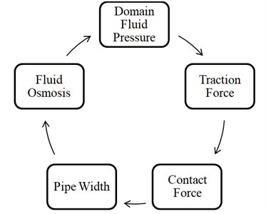
According to the above theories of fluid calculation, the traction force $F$ affects the contact force between the particles, while the $F$ is mainly determined by the fluid pressure $P$ in the domain. The change of the fluid pressure has a deep relationship with the seepage of the liquid flow. The rate of the seepage of the liquid flow is controlled by hydraulic aperture of the pipe. Finally, the hydraulic aperture is affected by the normal force at the contact point. Thus, there are three forms of the coupling between particles and fluid domains as below:

(1) The hydraulic pressure in the domain acts on the surrounding particles as the form of traction force, which will affect the contact force between the particles.

(2) The size of the hydraulic aperture is affected by the opening and closing of the contacts, which is determined by the contact force between the particles.

(3) The force on the contact between the particles can change the volume of the domain, causing the change of the liquid pressure in the domains.

In summary, the mechanism of fluid-mechanical coupling in PFC can be shown in the flowchart in below:

Fig. 2Flowchart of PFC mechanism of fluid-mechanical coupling

2.4. Modification of the algorithm

In order to make the numerical model closer to the actual situation, two modifications were made in the fluid-mechanical coupling based on the above calculation theories.

(1) In the actual hydraulic fracturing process, the seepage of the fluid will produce a lubricating effect with the surface of the fractures after cracking, which would weaken the frictional effect. Therefore, in this numerical model, the friction coefficient of the two particles at the contact in which the bond was broken down was set to zero [28].

(2) When a micro crack was formed since the bond of the contact was broken down, the hydraulic aperture of the pipe will be almost infinite, which will cause instability of the numerical model in the following fluid-mechanical coupling calculations. The simulation of fluid flow in these two domains connected by the failed bond plays an important role in hydraulic fracturing in PFC. Thus, the hydraulic pressure of the two adjacent domains connected by the failed bond were set to be equal, and both were equal to the larger value between the two domains. In this way, the infinite permeability could be ensured, so as to avoid the excessively large hydraulic aperture, resulting in a high rate of fluid flow exchange and shortening the time step to ensure the stability of the numerical model.

3. Establishment and verification of the numerical models

3.1. Establishment and verification of transversely isotropic rock masses model

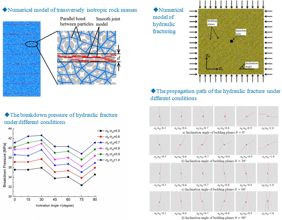
In this paper, a set of parallel smooth joint models (SJM) were embedded into the bonded-particle model (BPM) to simulate the mechanical properties of the transversely isotropic rock masses. At the same time, in order to better simulate the mechanical properties of the transversely isotropic rock masses, the bedding planes were simulated by embedding SJM within an area of certain thickness [29], as shown in Fig. 3. According to the experience in the research of Lei Xia [29], the thickness $d$ of the bedding planes area was taken as the diameter of the minimum particle, as shown in the Fig. 3.

Fig. 3Numerical model of transversely isotropic rock masses [29]

The macro-mechanical parameters of the Boryedong shale [30, 31] were taken as an example to build the uniaxial compression test specimens with the size of 50×100 mm. The minimum particle diameter was set as 0.6 mm, with the particle diameter ratio of 1.66. The particle size conformed to the Gaussian distribution, and the porosity of the model was taken as 0.16. A total of 5312 particles were generated in a single specimen and the microscopic parameters of the intact rock and smooth joints were shown in Table 1 and Table 2, respectively.

Table 1Microscopic parameters of intact rock

Ball parameters		Parallel bond parameters
Ball density [kg/m³]	2700	Modulus $\bar{E_{c}}$ [GPa]	39.0
Modulus $E_{c}$ [GPa]	39.0	Stiffness ratio $\bar{k_{n}}$ / $\bar{k_{s}}$	3.33
Stiffness ratio $k_{n}$ / $k_{s}$	3.33	Mean/SD normal strength [MPa]	95/9.5
Friction coefficient $μ$	0.8	Mean/SD shear strength [MPa]	95/9.5
Note*: (SD: standard deviation)

Table 2Microscopic parameters of smooth joint

Normal stiffness $k_{n, s j}$ [GPa/m]	Shear stiffness $k_{s, s j}$ [GPa/m]	Friction coefficient $μ_{s j}$	Normal strength $σ_{n, s j}$ [MPa]	Cohesion $C_{s j}$ [MPa]	Thickness $d$ [mm]
1200	700	0.4	25	25	0.6

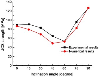
The comparison of the elastic modulus and uniaxial peak strength for specimens with different inclination angles of bedding planes between experimental and numerical results were shown in Fig. 4 and Table 3. It can be seen that both the elastic modulus and uniaxial peak strength of numerical results can be in good agreement with the experimental results under the above numerical modeling method and microscopic parameters.

Fig. 4Comparison between the experimental and numerical results: a) the elastic modulus, b) the uniaxial compressive strength

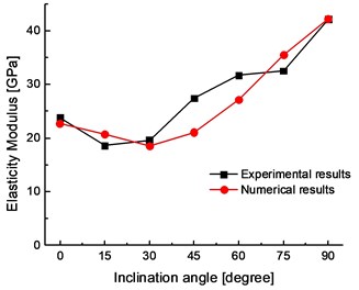
a)

b)

Table 3Comparison between the experimental and numerical result [30]

Macro-property		Inclined angle
Macro-property		0°	15°	30°	45°	60°	75°	90°
Lab	Elastic modulus [GPa]	23.8	18.6	19.6	27.4	31.7	32.5	42.1
Lab	UCS [MPa]	89.2	91.0	83.4	64.8	53.5	96.6	126.2
DEM	Elastic modulus [GPa]	22.68	20.79	18.50	21.06	27.18	35.53	42.14
DEM	UCS [MPa]	86.85	79.74	49.08	49.23	52.95	82.66	127.36

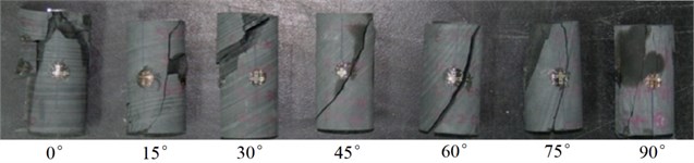
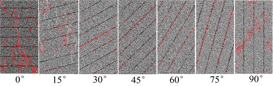
Meanwhile, the failure patterns of transversely isotropic rock masses from numerical models and laboratory experiments [30] with different inclination angles were compared in Fig. 5. The failure patterns in numerical models show an excellent agreement with the experimental results. For low inclination angle specimen (Inclination angle $θ =$ 0° and 15°), the failure was mainly occurred in the intact rock and the micro-cracks went through the bedding planes to form the macro-crack parallel to the direction of loading. When $θ =$ 30°-75°, the failure was mainly occurred along the bedding planes. The specimens damaged by the shear slip failure along some certain bedding planes. When $θ =$ 90°, due to no lateral confinement under uniaxial loading, the delamination failure occurred. The micro-cracks exist in both intact rock and bedding planes.

According to the comparison of macro-property and failure patterns of numerical simulation with experiments, the rationality of the numerical model had been verified.

Fig. 5Failure patterns of different inclination specimen: a) experimental results, b) numerical simulation results (the red color is the micro-crack, the black color is the bedding plane)

Failure patterns of different inclination specimen: a) experimental results, b) numerical simulation results (the red color is the micro-crack, the black color is the bedding plane)

a)

b)

3.2. Establishment and verification of hydraulic fracturing model

From the theory of the classical equations for stress concentration round a circular elastic borehole, which have been proposed by Hubbert [31], the breakdown pressure $P_{f}$ could be obtained as following expression:

5

P_{f} = 3 σ_{h} - σ_{H} - α P_{p} + S_{t},

where the $σ_{H}$ , $σ_{h}$ are the maximum and minimum principal stresses, $P_{p}$ is the pore pressure, $α$ is the effective stress coefficient and $S_{t}$ is the rock tensile strength.

In this paper, the size of the hydraulic fracturing numerical model was 1 m×1 m. In order to take account of the computing time, the minimum particle diameter of the numerical model was 6.0 mm, which made 18394 particles in a single specimen totally. The numerical example of hydraulic fracturing model for a special inclination of bedding planes was shown in Fig. 6. An injection hole was set in the center of the specimen, with a diameter of 15 mm. The space of the bedding planes was 70 mm. In the numerical model, the servo control system was established through the FISH codes to obtain different confining pressure, simulating different initial stress conditions.

Fig. 6Numerical model of hydraulic fracturing

$Numerical model of hydraulic fracturing$

At the same time, in order to better simulate the low tensile strength of the rock mass, the above microscopic strength parameters were set to relatively smaller values ( $σ_{n} = τ =$ 25 MPa, $σ_{n, s j} = C_{s j} =$ 7 MPa). The remaining microscopic parameters of BPM and SJM were the same as Table 1 and Table 2. With references of the previous research [21-25], the microscopic parameters in the fluid calculation were shown in Table 4.

Table 4Computational parameters for fluid

Parameters	Unit	Values
Initial hydraulic aperture	$a_{0}$ [m]	2.2×10^-6
Infinite hydraulic aperture	$a_{i n f}$ [m]	2.2×10^-5
Fluid dynamic viscosity	$μ$ [Pa·s]	1.0×10^-3
Bulk modulus of the fracturing fluid	$K_{f}$ [Pa]	1.0×10⁹
Injection rate	$R$ [m³·s^-1]	5.0×10^-5

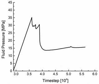
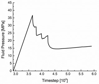
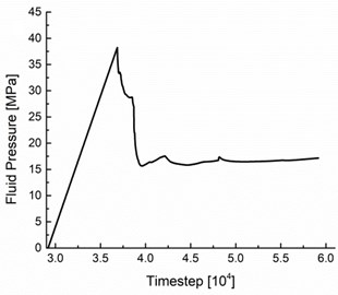
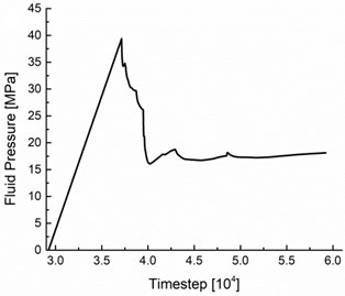
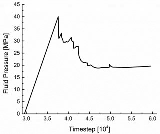
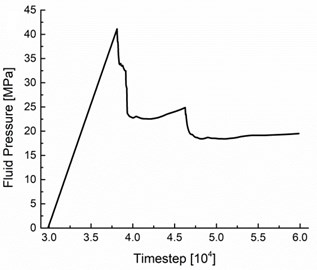
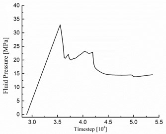
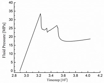
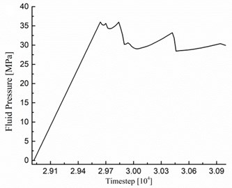
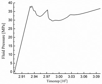
In order to verify the numerical model of hydraulic fracturing, hydraulic fracturing tests were carried out under different initial in-situ stresses. The inclination angle of the bedding planes was remained to 0°. The maximum principal stress $σ_{H}$ was kept unchanged ( $σ_{H} =$ 10 MPa), changing $σ_{h}$ to obtain different in-situ stress conditions. The fluid pressure history at the injection borehole during hydraulic fracturing simulation under different in-situ stress conditions was shown in Fig. 7.

Fig. 7The fluid pressure history at the injection borehole under different in-situ stress conditions: a) σh= 5 MPa, b) σh= 6 MPa, c) σh= 7 MPa, d) σh= 8 MPa, e) σh= 9 MPa, f) σh= 10 MPa

The fluid pressure history at the injection borehole under different in-situ stress conditions: a) σh= 5 MPa, b) σh= 6 MPa, c) σh= 7 MPa, d) σh= 8 MPa, e) σh= 9 MPa, f) σh= 10 MPa

a)

b)

c)

d)

e)

f)

As it can be seen from Fig. 7, the fluid pressure curves at the injection borehole were roughly similar to the ideal curve under different in-situ stress condition [32]. The rock mass around the borehole was broken because of the increasing injection pressure. And when the breakdown occurred, the flow volume would be lost, making the fluid pressure dropped steeply. The peak fluid pressure represented the crack breakdown condition. This implied a situation of unstable crack development, and the fluid entered the voids of cracks. Continued pumping would eventually result in stable crack growth, represented by the constant borehole fluid pressure level.

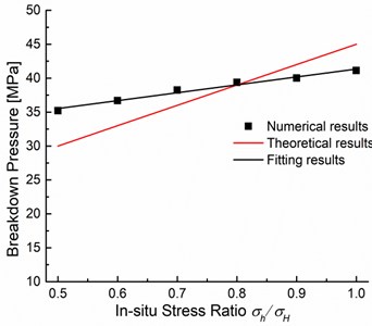
At the same time, as shown in Fig. 8, the crack breakdown pressure under different in-situ stress conditions from the numerical results were compared with Eq. (5). The numerical results showed that the breakdown pressure increased linearly with the increasing of the in-situ stress ratio, which was the same trend as the theoretical result of Eq. (5). These could prove the rationality of the mechanism of fluid-mechanical coupling in PFC.

Fig. 8Breakdown pressures obtained from numerical modeling and theoretical calculation based on Eq. (5) at different in-situ stress ratios

4. Numerical experiments

Based on the above numerical models, a series of hydraulic fracturing tests were conducted to study the influence of injection rates and in-situ stress ratios (the ratio of the maximum principle stress to the minimum one) on the initiation and propagation of the hydraulic fractures.

4.1. The influence of fluid injection rate

The fluid injection rate is a human controlled factor. To investigate the influence of injection rates on hydraulic fracturing characteristics, this paper utilized six different injection rates with unchanged fluid viscosity and in-situ stress condition. The in-situ stress condition was that $σ_{H} =$ 10 MPa, $σ_{h} =$ 5 MPa. And the numerical specimen with the bedding planes of 45° inclination angle was taken for the hydraulic fracturing tests.

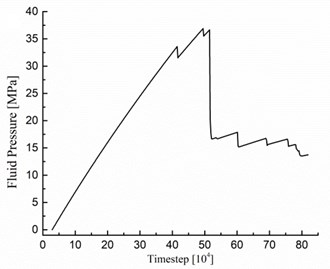
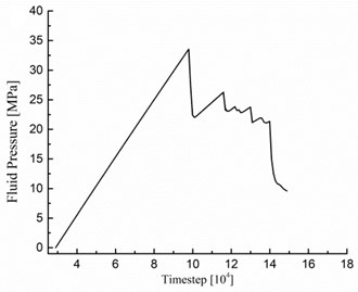
The fluid pressure history at the injection borehole during hydraulic fracturing simulation under different injection rates was shown in Fig. 9. And it showed that the crack breakdown pressure would increase once the injection rate was extremely small (1.0×10^-6 m³/s) or large (1.0×10^-3 m³/s), at which the crack breakdown pressure was 36.993 MPa and 38.159 MPa, respectively. As we know, faster fluid injection implied a higher strength similar to compressive tests of rock specimens applied with dynamic loads in the laboratory. Because stress in the solid skeleton induced by the injection borehole could not immediately adjust, higher fluid injection rate would lead to larger breakdown pressure in hydraulic fracturing [22]. What is more, when the injection rate reached to a large value (such as 5.0×10^-4 m³/s, shown in Fig. 9(e)), the fluid pressure in the borehole would not drop steeply after peak pressure. And a relatively high fluid pressure could be maintained to ensure stable crack growth.

Slower injection rate would make the injection time longer. Although the permeability of the reservoir rocks was extremely low in the numerical models, long-term injection would also cause sufficient time for the ‘fluid’ in the injection borehole to penetrate into the surrounding fluid domains. This allows the surrounding fluid domains to contain a certain hydraulic pressure, which would lead to increase the hydraulic crack breakdown pressure.

From an engineering perspective, excessively long-term injection severely affected the progress of the fracturing operations, and it also required a corresponding reduction in the pumping pressure of the injection. This may not achieve the desired purpose of hydraulic fracturing. On the other hand, with the excessively fast injection rate, crack initiation and propagation along multiple orientations were easily formed around the injection borehole [22]. Meanwhile, excessively fast injection rate would cause the situation that the original cracks were not widened and grown yet while the new crack initiation. This meant that the original and new cracks would not be penetrated to form an effective fracture network, which would greatly reduce the fracturing benefits.

Fig. 9The fluid pressure history at the injection borehole under different injection rates: a) R= 1.0×10-6 m3/s, b) R= 5.0×10-6 m3/s, c) R= 5.0×10-5 m3/s, d) R= 1.0×10-4 m3/s, e) R= 5.0×10-4 m3/s, f) R= 1.0×10-3 m3/s

The fluid pressure history at the injection borehole under different injection rates: a) R= 1.0×10-6 m3/s, b) R= 5.0×10-6 m3/s, c) R= 5.0×10-5 m3/s, d) R= 1.0×10-4 m3/s, e) R= 5.0×10-4 m3/s, f) R= 1.0×10-3 m3/s

a)

b)

c)

d)

e)

f)

4.2. The influence of in-situ stress ratio and inclination of bedding planes

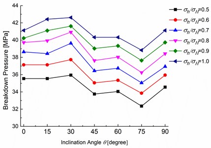
Both the initial in-situ stress condition and inclination angle of bedding planes are not human controlled factors. So, this section focused on the influence on the breakdown pressure and the propagation paths of hydraulic fractures. The injection rate was set to 1.0×10^-4 m³/s, and $σ_{H} =$ 10 MPa was kept constant. Taking six different initial in-situ stress condition ( $σ_{h}$ / $σ_{H} =$ 0.5, 0.6, 0.7, 0.8, 0.9 and 1.0) and seven different inclination angles of bedding planes ( $θ =$ 0, 15, 30, 45, 60, 75 and 90°) into account, a total of 42 hydraulic fracturing tests were conducted.

(1) The influence on the breakdown pressure.

The breakdown pressure of hydraulic fracture under different conditions was shown in Fig. 10. It can be seen that the breakdown pressure in the numerical models increased with the increasing in-situ ratio under different inclination angles of bedding planes. This result was the same as the Eq. (5). The change tendency of the initiation pressure with the inclination angles was basically the same in different in-situ ratios, which was increasing firstly, then decreasing and finally increasing, as a ‘wave’ type. And the increase extent was also the same with the increasing of in-situ ratios. The maximum breakdown pressure was taken when inclination angle $θ =$ 30°, while the minimum one was at $θ =$ 75°.

Because of the large spacing between the bedding planes in this research, the injection borehole did not intersect with the bedding planes. Therefore, the crack breakdown pressure was not reduced due to the influence of the intersecting bedding planes. The existence of bedding planes could affect the crack initiation direction around the injection borehole, and then resulted in different crack breakdown pressures.

Fig. 10The breakdown pressure of hydraulic fracture under different conditions

$The breakdown pressure of hydraulic fracture under different conditions$

(2) The influence on the propagation path.

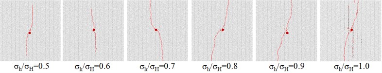
The propagation path of the hydraulic fracture under different conditions was shown in Fig. 11. Due to the space limitation, only the results when $θ =$ 0° (Fig. 11(a)), 30° (Fig. 11(b)), 60° (Fig. 11(c)) and 90° (Fig. 11(d)) were selected here, under different in-situ stress ratios.

Without considering the influence of the bedding planes, the minimum principal stress needed to be overcome, and then the hydraulic fractures will propagate along the direction of the maximum principal stress. As can be seen from the comparison of the different inclination angles of bedding planes, the existence of the bedding planes has a certain influence on the propagation path of the hydraulic fractures.

When the inclination angle was small (as shown in Fig. 11(a) and 11(b)), the propagation direction of the hydraulic fractures was deflected gradually with the increasing of the in-situ stress ratio $σ_{h}$ / $σ_{H}$ . When inclination angle $θ =$ 0°, only the relatively high in-situ stress condition ( $σ_{h}$ / $σ_{H} =$ 0.1-1.0) could induce the deflection of the propagation direction. And the hydraulic fractures would completely follow the direction of the bedding planes. When the inclination angle $θ =$ 30°, the smaller in-situ stress ( $σ_{h}$ / $σ_{H} =$ 0.6) could induce the change of the propagation direction. And even when $σ_{h}$ / $σ_{H} =$ 0.5, the propagation of the hydraulic fractures was also slightly deflected. However, due to the excessively large different degree of the in-situ stress when $σ_{h}$ / $σ_{H} =$ 0.5, the influence of the bedding planes was not large enough to change the eventual propagation, and the hydraulic fractures would still remain its original direction. When $θ =$ 30°, the direction of the hydraulic fractures was not completely along $σ_{H}$ when the crack initiated. This caused that the crack breakdown pressure was larger at $θ =$ 30° than other inclination angles of the bedding planes.

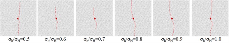
Fig. 11The propagation path of the hydraulic fracture under different conditions

$The propagation path of the hydraulic fracture under different conditions$

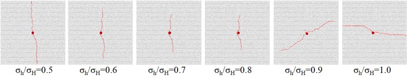
a) Inclination angle of bedding planes $θ =$ 0°

$The propagation path of the hydraulic fracture under different conditions$

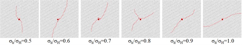
b) Inclination angle of bedding planes $θ =$ 30°

$The propagation path of the hydraulic fracture under different conditions$

c) Inclination angle of bedding planes $θ =$ 60°

$The propagation path of the hydraulic fracture under different conditions$

d) Inclination angle of bedding planes $θ =$ 90°

However, when the inclination angle $θ =$ 60-90° (as shown in Fig. 11(c) and 11(d)), the propagation direction of the hydraulic fractures hardly deflected with different in-situ stress conditions, and keeping propagated along $σ_{H}$ .

5. Conclusions

In this study, the bonded-particle element method with embedded smooth joints was applied to establish the transversely isotropic rock masses. The numerical simulation of hydraulic fracturing of transversely isotropic rock masses was carried out using the optimized fluid-mechanical coupling theory. The influence of the injection rate, in-situ stress condition and the inclination of the bedding planes on the initiation and propagation of the hydraulic fractures were preliminarily analyzed.

The numerical model of transversely isotropic rock masses was built by assembling the smooth joint models within a specific thickness region, with which the mechanical properties of the transversely isotropic rock masses can be better simulated. The fluid pressure history at the injection borehole during hydraulic fracturing simulation and the breakdown pressure under different in-situ stress condition were agree well with theoretical results, proving the rationality of the numerical modeling method of the fluid-mechanical coupling.

When injection rate was too large or too small, it would cause the increasing of the hydraulic crack breakdown pressure. When the injection rate was moderate, the crack breakdown pressure would remain at a relatively stable smaller value. The real distribution of joints and trend of bedding planes in the reservoir rocks are more complicated. According to the numerical results, combined with the actual engineering conditions, the most suitable injection rate would be selected to ensure the benefit of hydraulic fracturing.

Under different inclination angle of the bedding planes, the breakdown pressure of the hydraulic fracturing was correspondingly increased with the increasing of in-situ stress ratios. While under different in-situ ratio conditions, the breakdown pressure was in a change of ‘wave’ type with the increasing of the inclination angle of bedding planes. And the maximum breakdown pressure was at $θ =$ 30°, while the minimum one was at $θ =$ 75°. According to this conclusion, the optimal hydraulic fracture site could be selected based on the trend of bedding planes and current in-situ stress ratios.

The existence of the different inclination angles had a great impact on the propagation of the hydraulic fractures. The degree of the impact was different under different in-situ stress ratios. With the increasing of the in-situ ratio and when it trended to 1.0, the influence of the in-situ ratio on the crack propagation would be weaker and weaker, and the impact of the bedding planes would induce the hydraulic fractures to propagate in the direction of the bedding planes. The larger of the inclination angles, the more obvious of the deflective effect on the propagation of the hydraulic fractures. And due to the strong influence of the inclination angles, the propagation direction of the hydraulic fractures hardly deflected with different in-situ stress conditions, and keeping propagating along $σ_{H}$ . Meanwhile, the formation of the hydraulic fracture network could be reasonably controlled with the impact of different inclination angles on the propagation of the hydraulic fractures.

In this paper, the particle flow numerical model embedding the fluid-mechanical coupling mechanism was demonstrated to be a useful and strong tool for understanding hydraulic fracturing behavior. And hydraulic fracturing process should be studied in detail by means of modified particle flow numerical model in the future.

References

Jia L., Chen M., Sun L., et al. Experimental study on propagation of hydraulic fracture in volcanic rocks using industrial CT technology. Petroleum Exploration and Development, Vol. 40, Issue 3, 2013, p. 405-408.

Publisher
Zuo Y., Zhang S., Tong Z., et al. Experimental investigation into hydraulic fracture network propagation in gas shales using CT scanning technology. Rock Mechanics and Rock Engineering, Vol. 49, Issue 1, 2016, p. 33-45.

Publisher
Stanchits S., Burghardt J., Surdi A. Hydraulic fracturing of heterogeneous rock monitored by acoustic emission. Rock Mechanics and Rock Engineering, Vol. 48, Issue 6, 2015, p. 2513-2527.

Publisher
Heng S., Yang C. H., Guo Y. T., et al. Influence of bedding planes on hydraulic fracture propagation in shale formations. Chinese Journal of Rock Mechanics and Engineering, Vol. 34, Issue 2, 2015, p. 228-237.

Search CrossRef
Mcclure M. W. Modeling and Characterization of Hydraulic Stimulation and Induced Seismicity in Geothermal and Shale Gas Reservoirs. Ph.D. Thesis, Stanford University, Stanford, USA, 2012.

Search CrossRef
Kresse O., Weng X., Gu H., et al. Numerical modeling of hydraulic fractures interaction in complex naturally fractured formations. Rock Mechanics and Rock Engineering, Vol. 46, Issue 3, 2013, p. 555-568.

Publisher
Wang H. Y. Numerical modeling of non-planar hydraulic fracture propagation in permeable medium using XFEM with cohesive zone method. Journal of Petroleum Science and Engineering, Vol. 135, 2015, p. 127-140.

Publisher
Zeng Q. D., Yao J. Numerical simulation of multiple fractures simultaneous propagation in horizontal wells. Acta Petrolei Sinica, Vol. 36, Issue 12, 2015, p. 1571-1579.

Search CrossRef
Chen Z. Finite element modelling of viscosity-dominated hydraulic fractures. Journal of Petroleum Science and Engineering, Vol. 88, Issue 89, 2012, p. 136-144.

Publisher
Wang Y., Li X., Wang J. B., et al. Numerical modeling of stress shadow effect on hydraulic fracturing. Natural Gas Geoscience, Vol. 26, Issue 10, 2015, p. 1941-1950.

Search CrossRef
Yan C. Z., Zheng H., Sun G. H., et al. A 2D FDEM-flow method for simulating hydraulic fracturing. Chinese Journal of Rock Mechanics and Engineering, Vol. 34, Issue 1, 2015, p. 67-75.

Search CrossRef
Yan C., Zheng H., Sun G., et al. Combined finite-discrete element method for simulation of hydraulic fracturing. Rock Mechanics and Rock Engineering, Vol. 49, Issue 4, 2016, p. 1389-1410.

Publisher
Yan C. Z. A new two-dimensional FDEM-flow method for simulating hydraulic fracturing. Rock and Soil Mechanics, Vol. 38, Issue 6, 2017, p. 1789-1796.

Search CrossRef
Zhang X. P., Wong L. N. Y. Cracking processes in rock-like material containing a single flaw under uniaxial compression: a numerical study based on parallel bonded-particle model approach. Rock Mechanics and Rock Engineering, Vol. 45, Issue 5, 2011, p. 711-737.

Publisher
Potyondy D. O., Cundall P. A. A bonded-particle model for rock. International Journal of Rock Mechanics and Mining Sciences, Vol. 41, Issue 8, 2004, p. 1329-1364.

Publisher
Li X. F., Li H. B., Xia X., et al. Numerical simulation of mechanical characteristics of jointed rock in direct shear test. Rock and Mechanics, Vol. 37, Issue 2, 2016, p. 583-591.

Search CrossRef
Kong X. X., Liu Q. S., Zhao Y. F., et al. Numerical simulation on the effect of joint orientation on rock fragmentation by TBM disc cutters. Journal of China Coal Society, Vol. 40, Issue 6, 2015, p. 1257-1262.

Search CrossRef
Yoon J. S., Zimmermann G., Zang A. Numerical investigation on stress shadowing in fluid injection-induced fracture propagation in naturally fractured geothermal reservoirs. Rock Mechanics and Rock Engineering, Vol. 48, Issue 4, 2015, p. 1439-1454.

Publisher
Xia L., Zeng Y. W., Jin L., et al. Research on influence of initial horizontal principle stress on stress shadow. Chinese Journal of Rock Mechanics and Engineering, Vol. S1, 2016, p. 2819-2825.

Search CrossRef
Yang Y., Chang X. L., Zhou W., et al. Simulation of hydraulic fracturing of fractured rock mass by PFC2D. Journal of Sichuan University (Engineering Science Edition), Vol. 44, Issue 5, 2012, p. 78-85.

Search CrossRef
Chong Z., Li X., Chen X. Effect of injection site on fault activation and seismicity during hydraulic fracturing. Energies, Vol. 10, Issue 10, 2017, p. 1619.

Publisher
Zhang L., Zhou J., Han Z. Hydraulic fracturing process by using a modified two-dimensional particle flow code - case study. Progress in Computational Fluid Dynamics, Vol. 17, Issue 1, 2017, p. 13-26.

Publisher
Chong Z., Karekal S., Li X., et al. Numerical investigation of hydraulic fracturing in transversely isotropic shale reservoirs based on the discrete element method. Journal of Natural Gas Science and Engineering, Vol. 46, 2017, p. 398-420.

Publisher
Wang T., Zhou W., Chen J., et al. Simulation of hydraulic fracturing using particle flow method and application in a coal mine. International Journal of Coal Geology, Vol. 121, Issue 1, 2014, p. 1-13.

Publisher
Wang T., Hu W., Elsworth D., et al. The effect of natural fractures on hydraulic fracturing propagation in coal seams. Journal of Petroleum Science and Engineering, Vol. 150, 2017, p. 180-190.

Publisher
Cundall P. A. Fluid Formulation for PFC2D. Itasca Consulting Group, Minneapolis, USA, 2000.

Search CrossRef
Zhou J., Zhang L., Braun A., et al. Numerical modeling and investigation of fluid-driven fracture propagation in reservoirs based on a modified fluid-mechanically coupled model in two-dimensional particle flow code. Energies, Vol. 9, Issue 9, 2016, p. 699.

Publisher
Yoon J. Hydro-Mechanical Coupling of Shear-Induced Rock Fracturing by Bonded Particle Modeling. Ph.D. Thesis, Seoul National University, Seoul, Korea, 2007.

Search CrossRef
Xia L., Zeng Y. W. Parametric study of smooth joint parameters on the mechanical behavior of transversely isotropic rocks and research on calibration method. Computers and Geotechnics, Vol. 98, 2018, p. 1-7.

Publisher
Park B., Min K. B. Bonded-particle discrete element modeling of mechanical behavior of transversely isotropic rock. International Journal of Rock Mechanics and Mining Sciences, Vol. 76, 2015, p. 243-255.

Publisher
Cho J. W., Kim H., Jeon S., et al. Deformation and strength anisotropy of Asan Gneiss, Boryeong Shale, and Yeoncheon Schist. International Journal of Rock Mechanics and Mining Sciences, Vol. 50, Issue 2, 2012, p. 158-169.

Publisher
Hubbert M. K. Mechanics of hydraulic fracturing, Petroleum Transactions. AIME, Vol. 210, 1957, p. 153-168.

Publisher
Chen M., Jin Y., Zhang G. Q. Rock Mechanics of Petroleum Engineering. Science Press, Bejing, 2008, p. 41-43.

Search CrossRef

Cited by

Asymmetric failure mechanisms of anisotropic shale under direct shear

(2024)

Strength reduction model for jointed rock masses and peridynamics simulation of uniaxial compression testing

(2021)

Hydraulic fracture propagation barriers induced by weak interfaces in anisotropic rocks

Humberto M. Celleri | Martín Sánchez

(2021)

Hydraulic fracturing in transversely isotropic tight sandstone reservoirs: A numerical study based on bonded-particle model approach

Qi Zhang | Xiao-Ping Zhang | Wei Sun

(2020)

Hydromechanical bond-based peridynamic model for pressurized and fluid-driven fracturing processes in fissured porous rocks

Xiao-Ping Zhou | Yun-Teng Wang | Yun-Dong Shou

(2020)

About this article

Received

10 May 2018

Accepted

15 November 2018

Published

30 June 2019

DOI

https://doi.org/10.21595/jve.2018.19962

Keywords

transversely isotropic rock masses

hydraulic fracturing

fluid-mechanical coupling

particle flow code

breakdown pressure

crack propagation

Acknowledgements

This research is supported by funding from the National Natural Science Foundation of China (41272342, 51409013, 41772308).

This is an open access article distributed under the Creative Commons Attribution License, which permits unrestricted use, distribution, and reproduction in any medium, provided the original work is properly cited.

Previous article in issue Previous Next article in issue Next

Research article

2023 05 18

Optimization of process parameters for acid fracturing assisted herringbone well SAGD

Xi Yi, Guangsheng Cao, Jiaqi Tang

Research article

2021 06 21

A holistic review on hydraulic fracturing stimulation laboratory experiments and their transition to enhanced geothermal system field research and operations

C. Langbauer, F. Fazeli Tehrani, B. Mastobaev

Research article

2020 03 31

Seismic dynamic responses of earth-rock dam considering wave and seepage

Wei Jing, Jingxuan Wang

Research article

2019 06 30

Numerical investigation on rules of fracture propagation during hydraulic fracturing in heterogeneous coal-rock mass

Zhigang Yuan, Yaohua Shao, Donghai Xie, Fei Huang

L. Xia and Y. Zeng, “Numerical simulation of hydraulic fracturing in transversely isotropic rock masses based on PFC-2D,” Journal of Vibroengineering, Vol. 21, No. 4, pp. 833–847, Jun. 2019, https://doi.org/10.21595/jve.2018.19962

Copy Extrica

Copied to clipboard!

TY  - JOUR
DO  - 10.21595/jve.2018.19962
UR  - https://doi.org/10.21595/jve.2018.19962
TI  - Numerical simulation of hydraulic fracturing in transversely isotropic rock masses based on PFC-2D
T2  - Journal of Vibroengineering
AU  - Zeng, Yawu
AU  - Xia, Lei
PY  - 2019
DA  - 2019/06/30
PB  - JVE International Ltd.
SP  - 833-847
IS  - 4
VL  - 21
SN  - 1392-8716
SN  - 2538-8460
ER  - 

Copy Ris

Copied to clipboard!

@article{Zeng_2019,
	doi = {10.21595/jve.2018.19962},
	url = {https://doi.org/10.21595/jve.2018.19962},
	year = 2019,
	month = {jun},
	publisher = {{JVE} International Ltd.},
	volume = {21},
	number = {4},
	pages = {833--847},
	author = {Yawu Zeng and Lei Xia},
	title = {Numerical simulation of hydraulic fracturing in transversely isotropic rock masses based on {PFC}-2D},
	journal = {Journal of Vibroengineering}
}

Copy Bibtex

Copied to clipboard!

[1]Y. Zeng and L. Xia, “Numerical simulation of hydraulic fracturing in transversely isotropic rock masses based on PFC-2D,” Journal of Vibroengineering, vol. 21, no. 4, pp. 833–847, Jun. 2019, doi: 10.21595/jve.2018.19962.

Copy IEEE

Copied to clipboard!

Zeng, Yawu, and Lei Xia. “Numerical Simulation of Hydraulic Fracturing in Transversely Isotropic Rock Masses Based on PFC-2D.” Journal of Vibroengineering 21, no. 4 (June 30, 2019): 833–47. https://doi.org/10.21595/jve.2018.19962.

Copy Chicago

Copied to clipboard!

Numerical simulation of hydraulic fracturing in transversely isotropic rock masses based on PFC-2D

Abstract

Highlights

1. Introduction

2. Mechanism of fluid-mechanical coupling in PFC

2.1. Basic assumptions

2.2. Calculating theories

2.3. Fluid-mechanical coupling

2.4. Modification of the algorithm

3. Establishment and verification of the numerical models

3.1. Establishment and verification of transversely isotropic rock masses model

3.2. Establishment and verification of hydraulic fracturing model

4. Numerical experiments

4.1. The influence of fluid injection rate

4.2. The influence of in-situ stress ratio and inclination of bedding planes

5. Conclusions

References

Cited by

About this article

Related Articles